Results & Visualization Blog Posts
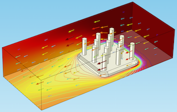
Plotting the Algebraic Residual to Study Model Convergence
Learn how to use the residual operator to plot the algebraic residual of your model, as well as visualize and understand the convergence properties of turbulent flow simulations.
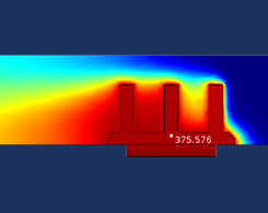
Using Annotation Plots in Your 2D and 3D Plot Groups
You can label the plots of your simulation results with names, comments, and values of quantities evaluated at specified locations. How? By adding annotation plots!
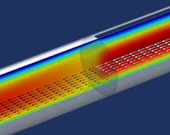
Analyze Thin Structures Using Up and Down Operators
Modeling complex geometries with thin structures can be very costly in terms of computational effort. Up and down operators are a way to efficiently and accurately compute these models.
Postprocessing Local Data Using Component Coupling
Derive numerical values. Create new coordinate systems. Link different components in the same model. How can you accomplish all of these tasks? By using Component Coupling operators.
Useful Tools for Postprocessing in COMSOL Multiphysics
Layering plots; style inheritance; enabling and disabling grids, axes, and legends; showing mesh plots, and more: We go over some useful tools for postprocessing your simulation results.
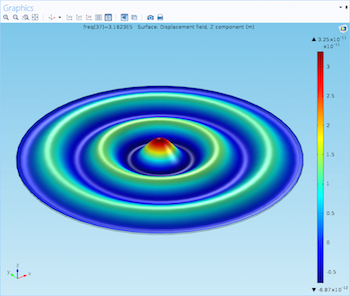
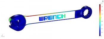
Using Deformations to Visualize Physical Motion
Postprocessing and visualization can help enhance your understanding of simulation results, and using plots to illustrate physical motion allows you to put everything into perspective.
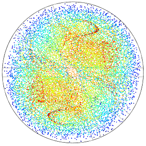
Application-Specific: Polar, Far-Field, and Particle Tracing Plots
When postprocessing your electromagnetics models, you can use polar, far-field, and particle tracing plots to effectively display your results. Learn how to use these 3 plot types here.
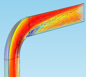
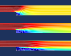
Visualizing Fluid Flow with Streamline Plots
As part of our blog series on postprocessing, we demonstrate the use of streamlines to visually describe fluid flow in your simulations. Learn how with an example of flow through a pipe elbow.