

When structures experience an excessive amount of compressive stress (i.e., when the load becomes critical), they deform due to an instability called buckling. To see how these deformations will affect a design, engineers not only study what happens at the critical load point but also what happens after it. With the COMSOL® software, they can accurately and efficiently perform a postbuckling analysis, which is demonstrated here using a spherical cap model, with results that have been verified with published research.
What Happens to a Structure During and After Buckling?
Buckling is a phenomenon in which compressive stress causes sudden failure in a structure. This instability can happen in a wide range of geometries, such as beams, plates, spheres, and cylinders. You may have seen this effect as “sun kink”, in which extreme heat causes railways to buckle, as well as deformations in pipes and even empty soda cans.


A cylindrical soda can before (left) and after (right) buckling.
In order to study buckling behavior, engineers typically perform a linear buckling analysis to predict the critical load. However, this analysis is limited. First, while it can help determine the buckling shape, it does not account for all of the displacements and stresses. Thus, it may be more accurate to perform a nonlinear buckling analysis, which applies the load gradually. Second, a linear buckling analysis doesn’t say what happens when the load is higher than the critical load. Often, a structure will still be able to support a load past the critical point without completely collapsing, but the deformations can be unpredictable and may affect surrounding structures or mechanisms (such as the buckling of a dome on a building). For these reasons, performing a nonlinear postbuckling analysis can be useful.
For such an analysis, using a displacement-controlled strategy (rather than a load-controlled one) is helpful. Take snap-through buckling, for example. In this phenomenon, a compressed shallow arch can “snap through” its base and undergo a deformation that reverses its shape. Snap-through buckling can happen in shallow arches and shells as well as truss structures like solar array panels and even MEMS devices. This effect occurs only after the critical load is reached, changing the structure into a new stable configuration (i.e., from an equilibrium state to a nonadjacent equilibrium configuration). For instance, after a convex, spherical cap (or other axisymmetric shell) experiences snap-through buckling, the displacement at the crown keeps increasing. Thus, a displacement strategy is needed to predict the snap-through behavior after that critical load point.
With the COMSOL Multiphysics® software and add-on Structural Mechanics Module, there’s a way to accurately and efficiently perform a postbuckling analysis. Let’s take a look at a simple spherical cap example that examines aspects such as the critical load and snap-through behavior, as well as softening and stiffening effects.
Modeling a Spherical Cap with a Central Point Load in COMSOL Multiphysics®
The verification model of a spherical cap is set up with a point load at its crown. As such, much of the focus is on the variation of the crown’s (center’s) axial displacement with respect to the applied load. In this example, the displacement at the crown increases monotonically, even with a decrease in load after a critical point in the snap-through region. To employ the displacement control strategy, you can apply a prescribed displacement in the COMSOL® software.
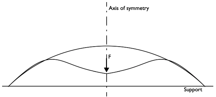
Spherical cap geometry with loading and boundary conditions.
The key to performing an efficient and accurate postbuckling analysis of an axisymmetric structure in COMSOL Multiphysics is the 2D axisymmetric Shell interface, available as of version 5.4. Just how efficient is it? To find out, you can set up the simulation to perform two studies, one with the Solid Mechanics interface and one with the Shell interface. For this model, 40 mesh elements are used for the first interface, as compared to the 4, 8, and 16 mesh elements with the second (solved for via a parametric sweep). The number of degrees of freedom is 406 using Solid Mechanics and 36, 68, and 132, respectively, using Shell. Note that with both physics interfaces, you can examine the snap-through behavior and softening effects for different displacements at the crown of the spherical cap.
Examining the Postbuckling Analysis Results for the Verification Example
First, let’s take a look at the total displacement at three different crown displacements. In the images below, you can see these displacements and their corresponding point loads. The three surfaces shown correspond to three different load levels. In both results, the top surface corresponds to the critical load, while the middle surface shows what happens after this load is reached. Even though deformation increases after the critical load point, the load itself decreases due to the softening effect. The bottom surface, meanwhile, shows the stiffening behavior after the snap-through phase, seen here as an increase in both displacement and load.
These results closely match the reference data (you can view this data in the tutorial documentation). When comparing the Solid Mechanics and Shell interfaces (with 40 and 16 mesh elements, respectively), the results are similar. However, the Shell interface is more efficient, as the mesh isn’t as fine, which leads to a reduced computational time.


Total displacement computed with the Solid Mechanics interface using 40 mesh elements (left) and the Shell interface using 16 mesh elements (right).
Results from this simulation can also help you compare the variation of the axial displacement at the crown to the applied load, as shown below. You can see that again, the Shell interface with 8 and 16 elements closely matches the Solid Mechanics interface while using far fewer mesh elements. The results for the Shell interface with 4 elements show that this is too few to replicate the solid model, similar to the reference values. However, the simulations with 8, 16, and 40 mesh elements closely match the reference values. What’s more, when you compare the solutions provided by the Shell interface in the image below, you can see that these results perform significantly better than the results from the reference. This is because while there are a multitude of possible shell element formations, the one used in the COMSOL® software is more efficient.
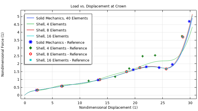
Applied load versus center displacement.
As demonstrated, you can accurately and efficiently perform a postbuckling analysis with the Shell interface in the COMSOL® software, including simulating the nonunique force and displacement relation as well as accounting for nonlinear deformation.
Next Steps
Try this verification model of a spherical cap by clicking the button below. Doing so will take you to the Application Gallery, where you can download the tutorial documentation and the MPH-file.
For a more advanced postbuckling example, where neither displacement nor force are monotonic, download the Postbuckling Analysis of a Hinged Cylindrical Shell model.


Comments (0)