
The laser is one of the most useful inventions in modern science, but it is not an easy device to use. Lasers work only when the cavity mirrors are aligned perfectly. Even if a laser is lasing for a while, it can stop all of a sudden. In today’s blog post, we will talk about how to predict laser stability using the ray-tracing capabilities in the COMSOL Multiphysics® software.
Introduction to Laser Simulation
Albert Einstein discovered stimulated emission in 1916, but the laser was invented by one of three American scientists, C.H. Townes, A.L. Schawlow, or G. Gould, presumably in 1957. (There was a patent war over who first theoretically invented the laser and there is still controversy about who came up with the idea.) The first laser was built by Theodore Maiman in 1960.
Lasers are very useful in many applications, such as cutting, perforation, melting, ablation, telecommunication, measurement, and spectroscopy among others. In the 1960s, A.G. Fox, T. Li, and H. Kogelnik made further progress in the research of lasers by coming up with ways to calculate the field distribution, formulate Gaussian beams, and predict the laser stability based on the paraxial theory of optics. These theories constituted the fundamentals for handling and designing lasers, even now, 60 years later.
Among the theories, Kogelnik’s laser stability theory is particularly useful for laser engineering. The theory consists of two parts:
- The paraxial wave optics theory predicts what Gaussian beam is generated in a laser cavity
- The geometrical optics theory predicts when the laser beam stays stable in the cavity
A laser may stop working after it is turned on or pumped harder. This is due to the thermal lensing effect. The laser crystal is pumped by another light source or sources to cause the inversion population. This process generates undesired heat by the residual energy of the pump light that is not used to induce the stimulated emission. The undesired heat introduces an undesired change in the refractive index and causes bulging of the crystal surface.
Kogelnik’s theory covers laser cavities including a rod lens, which approximates the thermal lensing effect by parabola fitting the temperature distribution in the crystal.
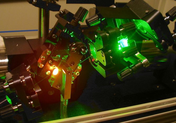
A titanium-doped sapphire femtosecond laser. The green laser from an Ar laser is used to pump the Ti:sapphire crystal emitting orange glare for the population inversion. The laser crystal is a circular rod, but has an angled cut called the Brewster cut. The pump beam enters the crystal surface at the Brewster angle to avoid undesired Fresnel reflections. Image by Hankwang — Own work. Licensed under CC BY-SA 3.0, via Wikimedia Commons.
Methods for Analyzing Laser Stability
The idea of the stability part of Kogelnik’s theory is quite simple: The laser beam is stable if a ray bouncing back and forth between the laser cavity mirrors does not escape from the cavity after a certain number of round trips. This theory was developed in a more concise and organized way by using the ABCD matrix theory based on paraxial optics rather than real ray tracing.
In this theory, thermal lensing is modeled as a thin lens that has a certain focal length. The focal length is calculated by fitting a parabola to the temperature distribution in the laser crystal. Thus, the ABCD matrix theory and the parabola fitting method are simple to perform and create beautiful results. You just need the distances of the optics, the focal length of any lenses involved, and the radius of curvature of the mirrors.
All folding mirrors are replaced by lenses having an equivalent focal length and an approximate focal length is used to represent the thermal lensing effect instead of giving the pump power in watts. Optics can’t be tilted and the optical layout is flattened to 1D in a straight line.
This method is too simple to handle more complex and more practical laser cavities. What if you want to see the results in 3D, or add a prism in your stability analysis? What if you want to fold your laser beam by folding mirrors, or tilt one of the optics? What about giving a pump power in watts, not an approximate focal length? Also, why not perform ray-tracing and thermal analyses without any restrictions or approximations?
Performing a laser stability analysis without taking the thermal lensing effect into account is almost useless, because every laser gets pumped. So, we need a thermal analysis as a counterpart of the stability analysis, which can’t be separated from ray tracing. By coupling the Heat Transfer and Geometrical Optics interfaces in COMSOL Multiphysics, we have all the tools we need.
Analyzing a Laser with a Confocal Cavity in COMSOL Multiphysics®
Let’s take a look at a simple example model of a laser cavity and briefly outline how the ABCD matrix method works and how it agrees with COMSOL Multiphysics results. This section complements part of one of Kogelnik’s own research papers (Ref. 1). In the ABCD matrix method, while following Hecht’s notation (Ref. 2), a ray is characterized by the ray angle θ and the ray position y in a 2×1 column vector as
\begin{array}{c}
\theta \\
y
\end{array}
\right ]
All optical processes including propagation, refraction, reflection, focusing, and defocusing are denoted by a 2×2 matrix called the ray transfer matrix.
For example, propagation through a distance L is denoted by a 2×2 matrix
\begin{array}{cc}
1 & 0 \\
L & 1
\end{array}
\right ]
and reflection in a mirror with the radius of curvature R in the air by
\begin{array}{cc}
-1 & -2/R \\
0 & 1
\end{array}
\right ]
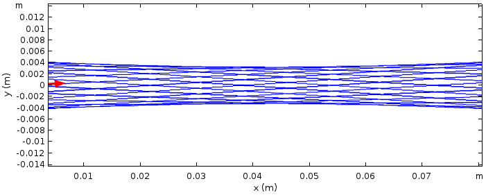
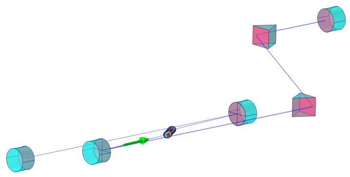
Our example laser cavity has a pair of identical mirrors that have the curvature of radius R = 0.1 m and cavity length L = R/2 = 0.05 m. This cavity looks like the below figure and is called the “confocal cavity”.
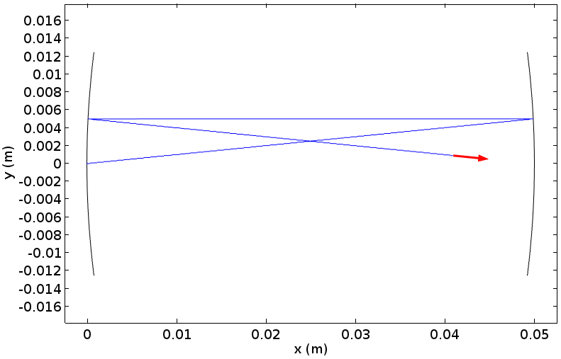
Ray tracing in COMSOL Multiphysics for a confocal cavity after a couple of bounces.
Let’s set θ0 = 0.1 rad and y0 = 0.01 m as the initial ray angle and position. (For the ABCD matrix method, the x-position really doesn’t matter, but let’s set the initial ray on x = 0 m; i.e., on the center of the left mirror.) The ABCD matrix method tells us that the next angle and the position of the ray after propagating the cavity length is calculated as
\begin{array}{c}
\theta_1 \\
y_1
\end{array}
\right ]
=
\left [
\begin{array}{cc}
1 & 0 \\
0.05 & 1 \\
\end{array}
\right ]
\left [
\begin{array}{c}
0.1 \\
0
\end{array}
\right ]
=
\left [
\begin{array}{c}
0.1 \\
0.005
\end{array}
\right ].
This is the ray angle and position on the right mirror (before it gets reflected). After the reflection, the next ray angle and position are still on the right mirror, but toward the left. They are calculated to be
\begin{array}{c}
\theta_2 \\
y_2
\end{array}
\right ]
=
\left [
\begin{array}{cc}
-1 & +20 \\
0 & 1 \\
\end{array}
\right ]
\left [
\begin{array}{c}
0.1 \\
0.005
\end{array}
\right ]
=
\left [
\begin{array}{c}
0 \\
0.005
\end{array}
\right ].
Then, another travel of the cavity length lets the ray return to the original left mirror as
\begin{array}{c}
\theta_3 \\
y_3
\end{array}
\right ]
=
\left [
\begin{array}{cc}
1 & 0 \\
-0.05 & 1 \\
\end{array}
\right ]
\left [
\begin{array}{c}
0 \\
0.005
\end{array}
\right ]
=
\left [
\begin{array}{c}
0 \\
0.005
\end{array}
\right ].
Finally, the end of one round-trip is the reflection by the left mirror; i.e.,
\begin{array}{c}
\theta_4 \\
y_4
\end{array}
\right ]
=
\left [
\begin{array}{cc}
-1 & -20 \\
0 & 1 \\
\end{array}
\right ]
\left [
\begin{array}{c}
0 \\
0.005
\end{array}
\right ]
=
\left [
\begin{array}{c}
-0.1 \\
0.005
\end{array}
\right ],
which can be confirmed in the above figure.
The beauty of this method is that you can only perform matrix operations to know the behavior of rays. We can calculate a matrix M that represents the sequence of the ray propagation and reflection as
\left [
\begin{array}{cc}
-1 & -20 \\
0 & 1 \\
\end{array}
\right ]
\left [
\begin{array}{cc}
1 & 0 \\
-0.05 & 1 \\
\end{array}
\right ]
\left [
\begin{array}{cc}
-1 & +20 \\
0 & 1 \\
\end{array}
\right ]
\left [
\begin{array}{cc}
1 & 0 \\
0.05 & 1 \\
\end{array}
\right ]
=
\left [
\begin{array}{cc}
-1 & -20 \\
0.05 & 0 \\
\end{array}
\right ],
which gives the same result as the previous result:
\begin{array}{c}
\theta_4 \\
y_4
\end{array}
\right ] =
\left [
\begin{array}{cc}
-1 & -20 \\
0.05 & 0 \\
\end{array}
\right ]
\left [
\begin{array}{c}
0.1 \\
0
\end{array}
\right ]
=
\left [
\begin{array}{c}
-0.1 \\
0.005
\end{array}
\right ].
This transfer matrix M has the property that M3 = I; i.e., it becomes the identical matrix after three round-trips. Actually, this can be proved analytically by means of Sylvester’s theorem without calculating a matrix product:
\begin{array}{cc}
A & B \\
C & D \\
\end{array}
\right ]^n
=
\frac{1}{\sin \Theta}
\left [
\begin{array}{cc}
A \sin n\Theta – \sin(n-1)\Theta & B \sin n\Theta \\
C \sin n\Theta & D \sin n\Theta – \sin(n-1) \Theta
\end{array}
\right ],
where \cos \Theta = (A+D)/2.
Substituting n = 3 in the above formula for our M matrix, we get M3 = I. We can confirm this with ray tracing in the next figure, in which the ray paths are colored by the number of round-trips.
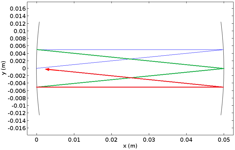
Ray-tracing results for the same confocal cavity as the previous plot, showing that the ray is returning to the initial position after 3 round-trips.
In this case, it is said that this cavity is stable, which means that the ray inside this cavity will not escape from it. The above formula is particularly useful for deriving a general consequence that the sequence represented by this matrix is stable when it holds for the trace of the matrix that -1 \le (A+D)/2 \le 1. In our case, the trace is calculated to (A+D)/2 = -1/2. So, it’s stable.
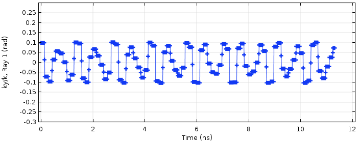
The results can be also viewed by plotting the y-component of the unit wave vector as in the below figure. The plot shows that the ray direction periodically alters but never grows and returns to the same value after 3 round-trips. Roughly speaking, ±0.15 radians is the upper and lower bound for the ray to be inside the cavity and the plot below indeed proves that this is the case here.
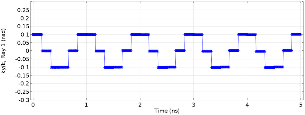
The y-component of the unit wave vector. The direction of the ray is bounded by a finite minimum and maximum, which means that the ray will not diverge beyond the cavity mirrors.
Changing the Laser’s Cavity Length
Let’s discuss another example. We’ll choose the cavity length to be L=R\left(1-\sqrt{1+\cos(9 \pi/10)/2} \right)=0.084357 m. This cavity is a little bit off from the confocal cavity. This intentionally tweaked cavity length guarantees that \sin(20\Theta)=0 and \sin(19\Theta)=-\sin(\Theta) in the formula. Therefore, the transfer matrix becomes the identical matrix after 20 round-trips and the initial ray angle and position are obtained. The transfer matrix in this case is
\begin{array}{cc}
-1.215 & -6.2574 \\
0.026393 & -0.68713 \\
\end{array}
\right ]
and the product of this transfer matrix for 20 times will be M20 = I. Let’s confirm this with ray tracing in the following figure. The red arrow is indeed back to the original mirror center and pointing to the original direction.
Ray-tracing results for a laser cavity with the same mirrors and a little longer cavity length after 20 round-trips.
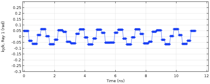
The y-component of the unit wave vector.
In general, the transfer matrix for the right mirror with the radius of curvature R1, the left mirror with R2, and the cavity length L for one round-trip is written as
\begin{array}{cc}
\left( -1+\frac{2L}{R_1} \right) \left( -1+\frac{2L}{R_2} \right) – \frac{2L}{R_2}
&
\frac{2}{R_1} \! \! \left( -1+\frac{2L}{R_2} \right) – \frac{2}{R_2}
\\
\left( -1+\frac{2L}{R_1} \right)(-L)+L
&
-\frac{2L}{R_1}+1
\\
\end{array}
\right ].
After some trivial arithmetic, the stability condition derived from the trace of the above matrix is expressed as
This stability formula is further extended to the case where a lens is involved in the cavity. Introducing a lens inside a cavity makes the transfer matrix complicated and it is no longer simple to write it out here, but the stability criterion is still simple. Adding a lens with focal length f modifies this to
where L0 = L1 + L2 – L1L2/f and L1 and L2 are the distance from the lens to the left and right mirrors, respectively. Let’s add a focusing lens with focal length f = 50 mm in the previous cavity, for which the stability criterion number is 0.10978, predicting that the cavity is stable.
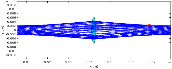
Ray-tracing results for the previous cavity with a thin lens added to it.
The y-component of the unit wave vector.
So far, we have studied some basic laser cavity stability analyses with the ABCD method side by side with the ray-tracing capabilities in COMSOL Multiphysics. The stability results from both approaches are in good agreement.
Simulating Lasers with Varying Focal Lengths
Now, let’s move on to the last example, in which the focal length in the previous example is parameterized and varied, and the variation of the cavity stability is plotted in the famous stability chart. In Kogelnik’s theory, the previous stability condition formula is rewritten as
by using a set of new variables defined by g1 = 1 – L2/f – L0/R1 and g2 = 1 – L1/f – L0/R2.
The stability regions are plotted as the hatched area in the following famous stability chart with g1 and g2 as the horizontal axis and the vertical axis, respectively. If g1 and g2, which are derived by the original cavity parameters R1, R2, and L0, are within the hatched area, the laser cavity is stable according to Kogelnik’s theory. For the previous example, we used the same radius of curvature for the two mirrors. So R1 = R2 and therefore L1 = L2 = L0/2 from symmetry, which results in g1 = g2. This is a 45-degree line. When the cavity parameters change, the values of g1 and g2 change along the line through the first and third quadrants.
Let’s take a look at how this is visualized. We fix the mirror curvature to 0.1 m and the cavity length to 0.084357 m while changing the focal length of the lens from 15 mm to 40 mm with 5-mm increments. The following figure shows Kogelnik’s theoretical results for this particular laser cavity with a lens. The laser is stable for f = 25, 30, 35, and 40 mm, giving g1g2 = 0.67091, 0.43100, 0.29200, and 0.20545, respectively.
These values are plotted in the hatched area, whereas the focal lengths of 15 and 20 mm make this laser unstable as their g1g2 values exceed 1.0; i.e., 1.1299 and 2.1593, respectively. The theoretical prediction for this laser cavity is plotted in the figure below. The ray-tracing result for each focal length is depicted in the sides of the figure showing a perfect match with the theory. In the COMSOL computation, the built-in stop condition terminates the computation once the ray gets out of the cavity. The ratio of the actual computation time T to the preset computation time T0 (50 ns in this case), T/T0 represents the cavity stability if T0 is appropriately chosen. Any value of this stability index other than 1.0 may not mean much, as we know that a real laser turns off really quickly when it gets unstable; in other words, the change of laser stability is almost digital, 1 (on) or 0 (off).

Comparison between Kogelnik’s stability theory and the COMSOL Multiphysics ray-tracing results for an off-confocal cavity with a thin lens.
This last example shows that ray tracing can perform a laser cavity stability analysis with the thermal lensing effect taken into account, since this example is Kogelnik’s model for a laser cavity with thermal lensing. In Kogelnik’s theory, a laser crystal heated by a pump laser is replaced by a thin lens with a certain focal length. Once the temperature distribution inside the crystal is known, the refractive index distribution is calculated by n = n0 + (T – T0)dn/dT to the first-order approximation, where n, n0 are the refractive index distribution with and without pumping; T, T0 are the temperature distribution with and without pumping; and dn/dT is the coefficient of index variation per temperature change.
The refractive index distribution of a pumped laser crystal is approximately a parabolic shape around the center if the crystal is a rod; i.e., n(r) = n0(1 – 2r2/a2), where r is the radial distance in the polar coordinate system with its z-axis along the optical axis of the pumping. The calculated refractive index distribution is fitted to this parabola to get the fitting parameter a. Once this parameter is calculated, the focal length that represents the thermal lensing effect can be approximated by f ~ a2/(4n0L), where L is the crystal length (Ref. 3). Thermal lensing also includes surface bulging, which causes refraction angle changes. This can be analyzed in a similar way.
Concluding Remarks
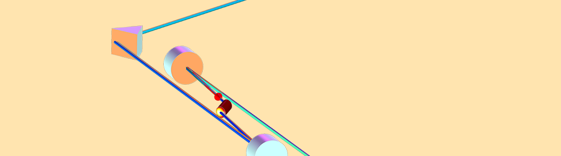
With COMSOL Multiphysics, we don’t have to do the fitting. We just do heat and mechanical simulation with the Heat Transfer and Solid Mechanics interfaces to know the new refractive index distribution and surface bulging and then simply carry out ray tracing with the ray optics interfaces to know the stability of your laser cavity under the thermal lensing effect. We will further discuss the ray-tracing capabilities of COMSOL Multiphysics in an upcoming blog post. Here, we see a full-fledged model analyzing the stability of a Ti:sapphire laser cavity with a double-pumped Brewster-cut crystal and a pair of dispersion compensation prisms. Stay tuned!
A stability analysis model for a Ti:sapphire laser cavity solving for temperature, mechanical displacement, and ray position and angle.
References
- H. Kogelnik and T. Li, Applied Optics, Vol. 5, No. 10 (1966)
- E. Hecht, Optics, Addison Wesley
- W. Koechner, Solid-State Laser Engineering, Springer
Additional Resources
- Browse these laser cavity tutorial models:
- Read more about laser simulation on the COMSOL Blog:

Comments (9)
Arne Heinrich
June 22, 2021Thank you for this very interesting article and it is impressive, what can be done. It would be very helpful, if you could attach the model file that we can test the capabilities in laser cavity design ourselves.
Yosuke Mizuyama
June 22, 2021 COMSOL EmployeeDear Arne,
Thank you for reading my blog.
Actually the basic model for analyzing the stability of a bow-tie laser cavity can be obtained from here:
https://www.comsol.com/model/bow-tie-laser-cavity-59771
Best regards,
Yosuke
Anju .
July 22, 2021Hii
Thank you for the article and it was explained very well. It could be very helpful if you could let me know how to model planoconcave mirrors instead of a concave or convex mirror.
Yosuke Mizuyama
July 22, 2021 COMSOL EmployeeDear Anju,
Thank you for reading my blog. You can just use any mirrors. Or, are you talking about modelling unstable laser cavities?
Best regards,
Yosuke
Anju .
July 22, 2021Thank you for the reply. I want to model stable laser cavities, and for that want to use a planoconcave mirror. However, in part libraries, there is a convex mirror and concave mirror only, planoconcave or planoconvex mirror not present. It could be very helpful if you could let me know how to proceed with this.
Yosuke Mizuyama
July 26, 2021 COMSOL EmployeeDear Anju,
There are plano-concave lenses in the Part libraries. You can just set the curved surface reflective.
Anju .
August 15, 2021Dear Sir
Thank you for the reply. I would like to know how to set conditions for using lens surface as reflective only.
Jakob Olsen
November 2, 2021Hi,
where can I find the heat and mechanical simulation?
Best regards
Jakob Olsen
Stephen Chinn
February 27, 2024I am interested in lasers whose active media (between plane mirrors) determine the mode parameters. Could you discuss COMSOL beam-propagation methods in such media where the combination of non-uniform gain guiding and thermal index guiding determine the mode solutions?