
Whenever ambient air is considered in an engineering context, temperature and moisture are intrinsically related. Vapor reaches a saturation point depending on the temperature and pressure conditions, while the action of latent heat modifies temperature distribution. These phenomena must be considered to optimize processes affected by phase changes, particularly when trying to prevent condensation occurring in devices. Let’s see how to model heat and moisture transport in air with the COMSOL Multiphysics® software.
Modeling Heat Transfer in Moist Air
Humidified air not only affects human comfort, but also conditions the sustainability of buildings and the operation of electronic devices. This makes accounting for the presence of moisture critical when modeling heat transfer and phase change in ambient air surrounding equipment and in structures.
A standard variable used to quantify the amount of moisture in air is the relative humidity, φ. It expresses a relative state toward saturation and is the ratio between the vapor’s partial pressure in air, pv, and the saturation pressure at a given (usually standard) temperature, psat(T):
As a first approximation, we can assume the vapor’s partial pressure pv to be homogeneous. Yet, because of the dependence of saturation pressure on temperature, we should note that the relative humidity is not actually homogeneous, as temperature gradients are present.
Typical ambient moisture conditions can be defined from tabulated data such as weather records. These can be used to define, for example, the air’s thermodynamic properties when solving the heat transfer equation:
The moisture dependence on the density, thermal conductivity, and heat capacity at constant pressure are set through a mixture formula based on dry air and pure steam properties.
In a previous blog post, we detail how to use typical weather data for temperature and relative humidity in COMSOL Multiphysics®.
By exclusively solving the equation above for the temperature while knowing the (homogeneous) vapor’s partial pressure, we can already identify zones where condensation is likely to happen. Indeed, condensation happens at the saturation state, corresponding to φ = 1, where the detection of condensation relies on the relationship between both temperature and moisture.
As an example, let’s consider an electronic device within a box that produces 1 W of heat. Moist air flows through the box via 2 small slits located at the left and right sides of the box. From the computed temperature and relative humidity distributions, the risk of condensation inside the box is evaluated. Note that in this computation, the latent heat associated with the condensation is not accounted for in the heat transfer model. As shown in the figures below, condensation forms on the walls close to the slits after around 3 hours, for about 30 minutes, as well as after 4 hours and 30 minutes. These times correspond to when the ambient temperature is low and the relative humidity is high, at different points in the box.


Temperature distribution after 3 hours (left); relative humidity distribution after 3 hours (center); and the evolution of the condensation indicator variable, ht.condInd, over time (right).
You can find more information in a previous blog post on modeling convective heat transfer.
When using the Heat Transfer Module, the Moist Air option in the Fluid Settings window from the Heat Transfer in Fluids interface defines the moisture-dependent thermodynamic properties of the modeling domain. This option also provides the ht.condInd variable to be used when postprocessing results to identify condensation detection.
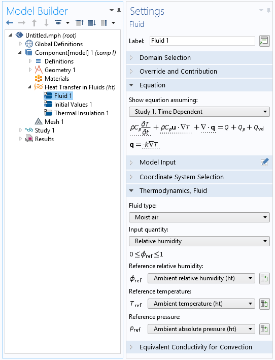
The model tree and Settings window of the Fluid feature with the Moist air option selected.
Coupled Modeling of Heat and Moisture Transport in Air
In some situations, we need to describe the moisture distribution more precisely. This includes cases where the amount of moisture is locally high due to evaporation and when the diffusion and convection of vapor can’t be neglected.
Compared to the previous approach, we need to compute the moisture distribution by solving an additional transport equation for the convection and diffusion of the vapor concentration cv in air:
Note that in this equation, the temperature dependence is still accounted for through the vapor concentration cv = φcsat(T), with csat(T) as the saturation concentration of vapor.
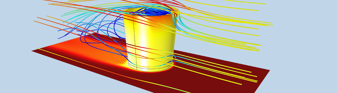
Let’s consider a beaker filled with hot water (80°C) and placed in an air flow with a velocity of 2 m/s. Evaporation occurs from the water surface due to the flow of the air. Evaporation creates a state of saturated vapor (dependent on the temperature) at the air-liquid water interface, where this is transported away, and replenished by unsaturated air through convection and diffusion (see the figure below).

Vapor concentration distribution after 20 minutes, with contour lines for the relative humidity.
The energy required to sustain the evaporation is primarily extracted from the internal energy of the liquid water, which cools down as a result, as shown in the animation below. This process is known as evaporative cooling. It is the main process used in evaporative coolers and cooling towers, taking advantage of water’s relatively large heat capacity and latent heat when heating and vaporizing water for air cooling.
Temperature distribution over time and streamlines indicating the flow field.
In the model, evaporation occurs when the vapor concentration stays below the saturation state and just above the liquid surface. The evaporation flux is expressed as:
where K is an evaporation rate depending on the application.
The latent heat variation in the liquid is taken into account by adding the following heat source in the heat transfer equation:
where Lv is the latent heat of the evaporation of water.
When using the Heat Transfer Module, the Heat and Moisture Transport interface adds the subnodes shown in the screenshot below, including the:
- Heat and Moisture coupling node
- Heat Transfer in Moist Air interface
- Moisture Transport in Air interface
- Moist Air feature for the heat transport in air
- Moist Air feature for the vapor transport in air
- Wet Surface feature for the evaporation from the liquid surface
- Boundary Heat Source feature, which adds the latent heat source due to evaporation to the heat transfer equation
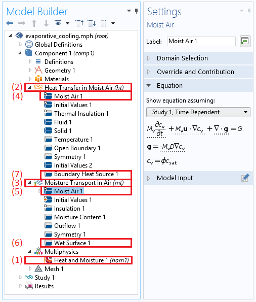
The model tree and subsequent subnodes when choosing the Heat Transfer in Moist Air interface, along with the Settings window of the Moist Air feature.
When defining a fully coupled simulation of evaporative cooling, the Heat Transfer in Moist Air and Moisture Transport in Air interfaces are included together with the Heat and Moisture multiphysics interface. This also sets up the situation by including the first three subnodes under both interfaces by default. Further subnodes (e.g., the Boundary Heat Source and Wet Surface subnodes) can be included depending on the participating conditions of the process being simulated.
Closing Remarks on How to Model Heat and Moisture Transport in Air
We have now reviewed the COMSOL® software features dedicated to the modeling of heat and moisture transport in moist air. Depending on the application, you may want to solve only for heat transfer and use the temperature prediction to detect condensation, or you may need to go further by computing the temperature and moisture distributions in a coupled way. In addition, you can account for the latent heat effects or disregard them. COMSOL Multiphysics (along with the Heat Transfer Module) provides the tools to define the corresponding models for a large range of applications.
Stay tuned for an upcoming blog post covering how to model heat and moisture transport in building materials and porous media.
Editor’s note: You can read the follow-up post in this blog series here: “How to Model Heat and Moisture Transport in Porous Media with COMSOL®“.
Try It Yourself
- Check out the tutorial models featured in this blog post:


Comments (9)
Omar Almahmoud
July 22, 2017I cannot find moisture transfer in air physics. Does really exist in COMSOL?
How-Ming Lee
June 5, 2018Thanks for a very good application. As you mentioned, “K” is an evaporation rate depending on the application. I had found that “K” significantly affects the evaporation amount and heat. Could you share how or where to find detail information on the evaporation rate. Thank you.
PS: In COMSOL’s examples, the “K” is always set as a constant. However, “K” should be varied with the time, since the temperature difference between the water pool and the gas is getting small.
Claire Bost
June 6, 2018Hi,
For the definition of K in function of the temperature, the Hertz-Knudsen equation may be used. It is based on the kinetic theory to express the mass flux on flat interfaces.
This expression can be set for the K user input.
Concerning the setting of K as a constant value, I don’t have any recommendation. Maybe starting from the Hertz-Knudsen equation and making some approximations can provide such a value?
Mehdi Amiri
June 6, 2018Thanks for a good blog post!
Regarding condensation on a flat plate, is there any COMSOL model that I can be referred to? I am interested in modeling evolution of water layer thickness condensated on a cold flat surface.
Regarding the question about K and its change with temperature, a possible way is to relate K to heat transfer coefficient (h) through Lewis Number (Le). Mass transfer coefficients (K) can estimated from the heat transfer coefficients (h) using the Lewis number (Le) that compares thermal and mass diffusivities, through the Chilton–Colburn analogy.
Claire Bost
June 7, 2018Hi,
Thanks for your input about the Chilton–Colburn analogy. Indeed this analogy is implemented since Version 5.3a in the Moisture Flux boundary condition. For a set of different flow (natural/forced convection) and geometry conditions, you can obtain the convective heat transfer coefficient from correlations based on Nusselt number, and the analogy is applied to compute the moisture transfer coefficient.
There is no COMSOL model solving for condensation on a flat plate. The “Evaporative cooling of water” model presented in this post would be the closest example.
Phong Huynh
September 6, 2018Thank you very much.
Omar Al-Rawi
October 1, 2018Hi,
Thank you for this good blog post.
Indeed, I have two quastions about this model. Can you please explain clearly what is the difference between modelling this application on COMSOL 5.3 and 5.3a?
I have noticed that instead of using “Transport of Diluted Species” as in 5.3 version, you used “Moisture Transport in Air”. What is the difference between these two physics interfaces?
And if I am trying to determine the evaporation rate from a liquid, could not I use the later interface?
Regards,
Omar
Claire Bost
October 2, 2018Hi Omar,
The Moisture Transport in Air interface is specially designed for the transport of water vapor in air. The Moist Air domain node (Moisture Transport in Air interface) solves for a particular case of the transport equation solved by the Transport Properties domain node (Transport of Diluted Species interface), when only one specie is considered. In particular, the diffusion coefficient D is preset in the interface. When considering moisture transport in building materials, the Building Material node can be added under the Moisture Transport in Air interface for some domains, and a single variable, the relative humidity phi, allows modeling moisture both in air and in the building material.
For this example you could as well use the Transport of Diluted Species interface.
In the Moisture Transport interface, the Wet Surface and Moist Surface boundary conditions make it possible to specify an evaporation rate. It is also possible to account for evaporation by using the Moisture Flux condition, by specifying some convective moisture flux, and account for it in the evaporation. The variable mt.g_evap gives access to the evaporation flux.
Best Regards,
Claire
Alan Collier
July 5, 2019Hi Claire,
I’m modelling how much time is required to equilibrate a closed atmosphere above a pool of water or salt solution at different temperatures, and your post has helped considerably! I have one question:
Since my system is closed and static, the water vapour transport is driven by diffusion alone, and I know that the diffusion constant varies significantly with temperature.
In your above comment to Omar, you point out that the diffusion coefficient is preset. Does this include a temperature term, or can one be incorporated into the model specfically?
Many thanks,
Alan