

Ion-exchange membranes are widely employed within the field of electrochemical engineering. In polymer electrolyte fuel cells and vanadium flow batteries, they are used to conduct ions and at the same time prevent reactants and electrons from crossing between the two flow compartments. The ability to promote the passage of ions of either positive or negative charge is also used in electrodialysis for cleaning water from ions. In this blog post, we will explore the ion-selective capabilities of ion-exchange membranes.
The Nernst-Planck-Poisson Equations
An ion-exchange material is typically modeled as a porous medium consisting of a fixed matrix with the pores filled up with water and additional mobile ions. This may sound completely wrong to anyone who has seen, for instance, a Nafion® membrane, one of the most common polymer electrolyte materials. This material looks perfectly transparent and homogeneous, but the matrix is made of a transparent polymer backbone. The pores, swelling when in contact with water, are in the range of nanometers.
The key feature of the ion-exchange membrane is the immobilized ions that are fixed to the backbone and located on the internal pore walls. In the case of Nafion®, the immobilized ions are \mathrm{SO}_3^- groups located at the end of polymer tails extending from the polymer backbone. As we will see in the following discussion, the concentration and sign of the fixed charge in the ion-exchange membrane is crucial for the ion transport of mobile ions in the membrane.
The Poisson equation relates the sum of all charges to the potential according to
(1)
where \phi_l is the electric potential of the electrolyte phase, \epsilon is the permittivity, and \rho is the space charge density.
In our case, we can split the space charge into the contributions from the mobile and immobile ions
(2)
where F is Faraday’s constant; z_i is the charge; c_i is the concentration of the mobile ions, where i is a species index and the summation is made over all N ions; and \rho_\textrm{fix} is the charge density of the immobilized ions in the matrix.
In a free electrolyte outside the ion-exchange media, the immobile ion concentration is zero so that \rho_\textrm{fix}=0.
To model the transport of ions, we first define the electrochemical potential for each ion as
(3)
where R is the molar gas constant, T is the temperature, and c_{i,\textrm{ref}} is some (arbitrary) reference concentration.
Assuming a dilute solution (i.e., each ion interacts with the surrounding water molecules only) and that ion transport only occurs due to diffusion and migration, we define the flux of the mobile ions based on the gradient of the electrochemical potential according to
(4)
where \mathrm{mob}_i is the mobility.
The flux of the immobilized ion is zero. Note that we would typically expect lower mobilities for the ions in the membrane compared to the free electrolyte due to porosity and tortuosity effects. However, we will ignore that in the following example.
If you are used to modeling diffusion by Fick’s law, it is also worth mentioning that the mobility and the diffusion coefficient are related by the Nernst-Einstein relation
(5)
Since there is neither production nor consumption of ions, and assuming a stationary solution, the divergence of the ion flux is zero.
(6)
Eq. (1) together with Eq. (6) (one for each species) is commonly referred to as the Nernst-Planck-Poisson (NPP) set of equations.
Modeling an Ion-Exchange Membrane with the NPP Equations
Let’s apply the NPP equations to a simple problem and investigate how the ion-selective capabilities vary as we vary the concentration of the fixed ion in the membrane.
As a modeling problem, we play around with a 100-μm-thick membrane surrounded by two free electrolyte domains of the same length and located in a 1D geometry. We model the transport of three ions — A+, B–, and C– — and we will also add a fixed charge to the middle ion-exchange membrane domain. At the leftmost and rightmost external boundaries, the concentrations and potentials are fixed. This model could, for instance, represent one of the membranes in an electrodialysis cell, where turbulence ensures good mixing, which allows us to assume constant concentrations outside the diffusion boundary layers on each side of the membrane (see Figure 1).
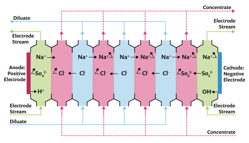
Figure 1. Schematic of an electrodialysis cell used for desalination of water. An ion-exchange membrane is located between each fluid compartment. The sign of the immobilized charge of the membrane, which alternates, will govern whether the membranes will predominantly allow passage for positive or negative ions.
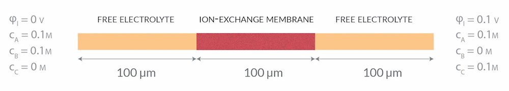
Figure 2. Geometry and boundary conditions.
On the left boundary, we set \phi_l = 0 V, c_A = 0.1 M, c_B = 0.1 M, and c_C = 0. On the right boundary, we set \phi_l = 0.1 V, c_A = 0.1 M, c_B = 0 M, and c_C = 0.1 M. The mobilities are set to be equal for all ions and we set the charge of the immobilized ion in the membrane to -1.
As we will see, using the NPP set of equations for modeling ion-exchange membranes results in increasingly steeper gradients for the dependent variables when increasing the fixed membrane charge. Therefore, we solve the problem, using a stationary solver, by ramping up the concentration of the immobilized ion from 0 to 1 M (using an auxiliary sweep in the COMSOL® software).
Figure 3 shows the molar flux for each ion through the cell (in the direction from left to right) when varying the immobilized ion concentration from 0 to 1 M. Regardless of the membrane charge, the direction of the electric field results in A+ being transported to the left (the flux having a negative sign).
The boundary condition for the concentrations of B– and C– determine the overall flux direction for these species, but the direction of the electric field explains why B– is transported to the right at a higher rate than C–, which is transported to the left. When increasing the membrane charge, we can see that the flux of B– decreases (and at close examination, C– as well); i.e., when increasing the membrane charge, this results in an increased blocking of both B– and C– for membrane transport. It should also be noted that the blocking is not complete.
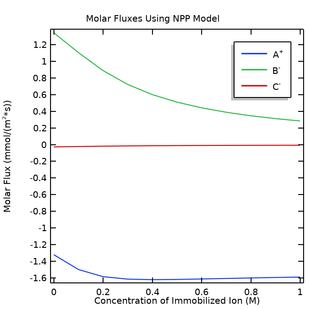
Figure 3. Molar fluxes through the cell for the mobile ions in the NPP model when varying the concentration of the immobilized ion in the membrane.
Plotting the concentrations for the NPP problem in Figure 4 reveals a crucial part in the explanation of the blocking effect. The concentration of A+ is higher in the membrane than in the surrounding free electrolyte, whereas the concentrations of B– and C– are suppressed. Returning to the flux definition in Eq. (4), we see that low ion concentrations of B– and C– have a negative impact on the flux; i.e., a low concentration results in blocking.
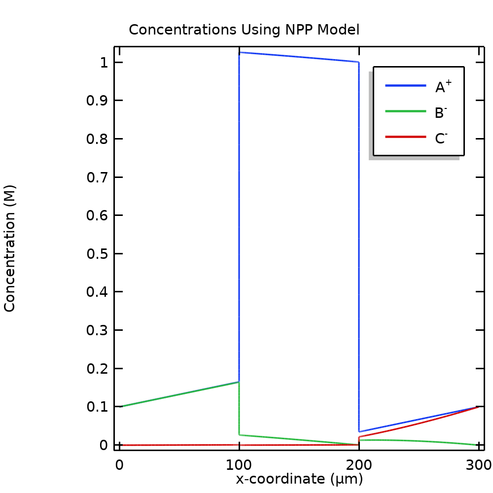
Figure 4. Molar concentrations of the mobile ions for the NPP model.
Why do we get an increase of A+ and a decrease of B– and C– in the membrane, with very steep gradients at the boundaries between the free electrolyte and the ion-exchange membrane? To find the answer, we return to Eq. (1). Inspecting this equation and keeping in mind that the permittivity is typically in the order of 10-12 (F/m), we see that any net space charge deviating from zero has a huge impact on the potential, unless the nonzero net charge is confined to a very small region in space. As a result, nonzero space charges are usually only found in very thin regions close to phase boundaries, such as an electrolyte-electrode interface or, as in this case, a membrane-free electrolyte interface. Assuming a zero space charge (electroneutrality) is hence usually a very good approximation for any electrolyte solution outside a nm-range of a phase boundary. Since A+ is the only positive ion in our system, and as a result of electroneutrality, the concentration of A+ increases to approximately match the charge of the immobilized negative ion in the ion-exchange domain.
Figure 5 shows the plot of the electrolyte potential in the NPP model. Similarly to the concentration shifts in Figure 4, we see significant potential shifts at the boundaries between the ion-exchange and the free electrolyte domains. Since the flux of all species is constant through the cell (Eq. (6)), the steep gradients of the potential are needed to balance the steep gradients in the concentrations. Since the sign is opposite for B– and C– compared to A+, the concentrations of B– and C– are suppressed in the membrane.
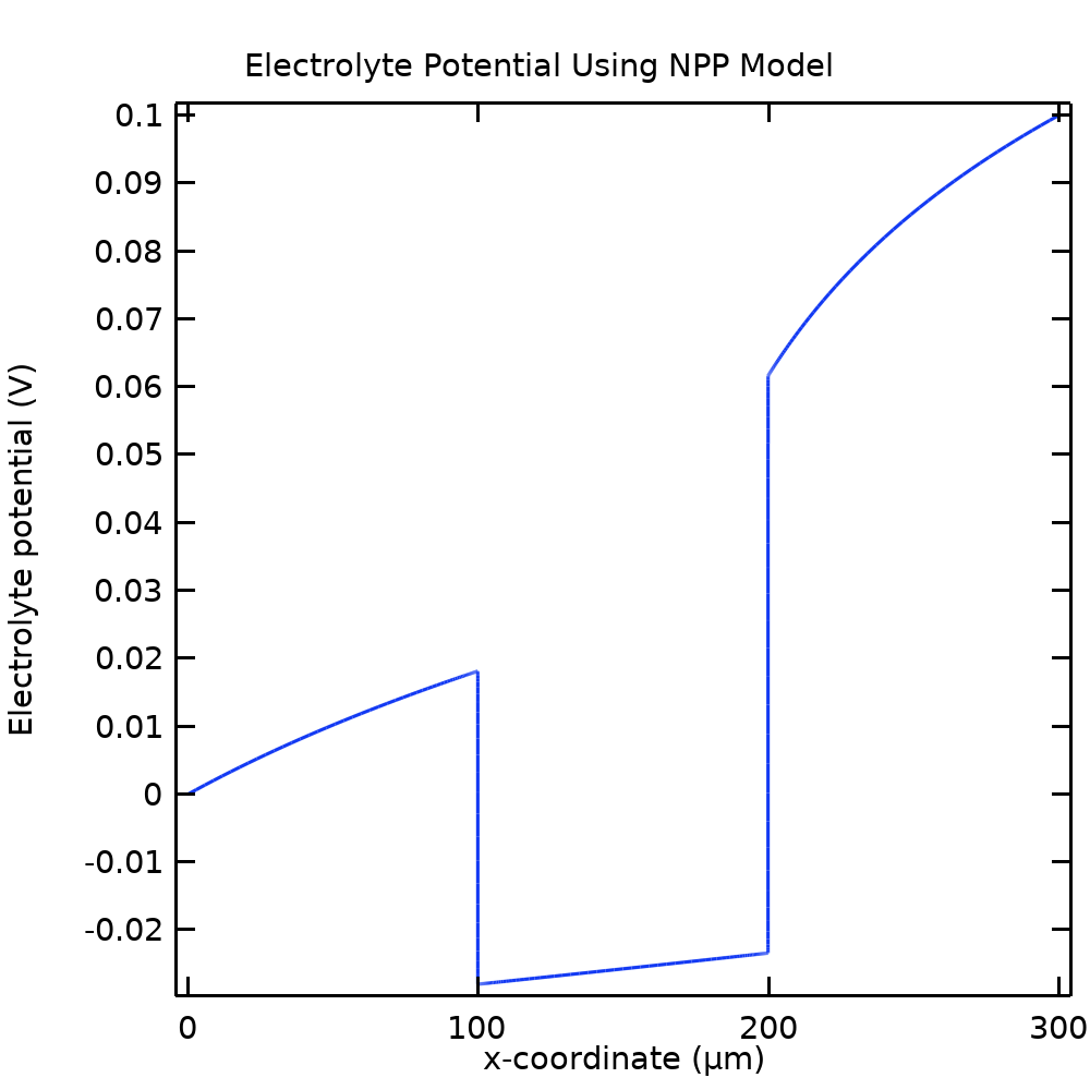
Figure 5. The electric potential of the electrolyte phase for the NPP model.
In both Figure 4 and 5, the concentration and potential gradients at the phase boundaries are extremely high: In the plots, they show up as vertical lines. This results in numerical difficulties, since the mesh in these transition regions needs to be well resolved. Zooming into either Figure 4 or 5 would reveal that the transition region has a thickness of around 1 nanometer, so typically, a mesh size in the subnanometer range is needed in order to resolve the gradients. The mesh used in this example consists of approximately 500 elements. For 1D simulations, this is usually not a problem. However, when modeling in higher dimensions, the requirement for a fine mesh may result in memory issues. Is there any way to circumvent these issues related to the transition region?
Introducing Donnan Potential Conditions and Electroneutrality
The answer is yes and comes from returning to the definition of the electrochemical potential in Eq. (3). Plotting the electrochemical potential of A+ in Figure 6 (using the concentration at the leftmost boundary as reference) reveals that this potential varies continuously through the cell, with no sharp gradients at the membrane-free electrolyte boundaries. (Plotting the electrochemical potential of B– and C– would also render fairly smooth curves).
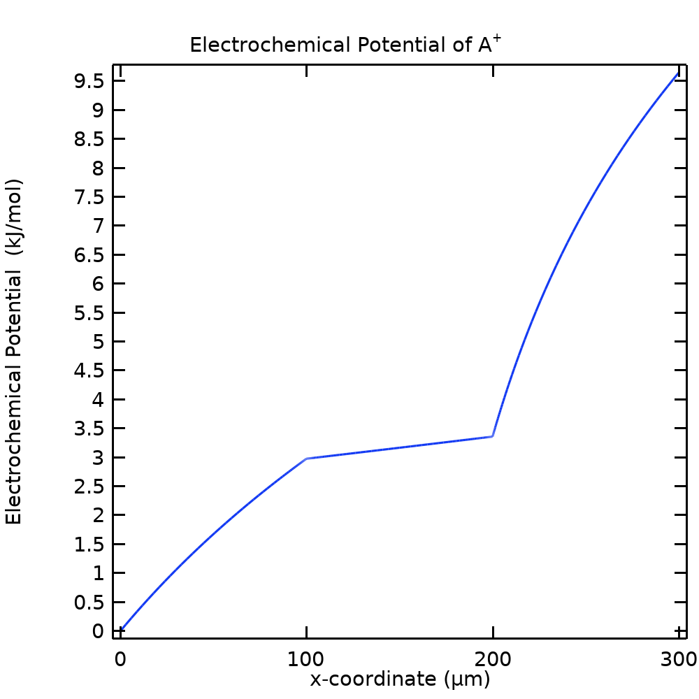
Figure 6. The electrochemical potential of A+ for the NPP model.
By assuming the electrochemical potential to be the same on each side outside of the transition region, it is possible to derive a relation between the ion concentrations and the potentials on each side of the interface according to
where we are using the arbitrary indices u and d to define the value on each side of the internal boundary.
This potential shift is called a Donnan potential. Donnan potentials provide one constitutive relation per mobile ion. By requiring continuity of the ion fluxes and the condition of electroneutrality, which is usually fulfilled outside a nm-length from a phase boundary, we can formulate a complete set of internal boundary conditions for all concentration variables and the electric potential on the membrane-free electrolyte boundaries. It should be stressed here that when using this formulation, we need dual instances of the dependent concentration and potential variables on the internal boundary, each representing the variable value when approaching the boundary from either the right or left, respectively. (This is called a slit condition in COMSOL Multiphysics®).
While we are at it, we can also replace the use of Poisson’s equation (Eq. (1)) in the domains by assuming electroneutrality everywhere, and instead derive a potential equation based on the sum of all species fluxes times their respective charges
(For convenience, we have also multiplied the sum by F so that we get an expression with the unit of A/m2; i.e., the total current density. In this way, Neumann boundary conditions may be expressed in this unit.)
This reduces the number of dependent concentration variables by 1. In this new equation system, we solve for N-1 concentration variables and the electric potential variable, keeping in mind that we can always derive the Nth concentration from the other concentrations and the condition of electroneutrality.
The reformulated model problem, using the condition of electroneutrality everywhere and Donnan potentials at the internal boundary, can be solved using far fewer mesh elements. Figure 7, plotting the same concentrations as Figure 4, shows the result when using only 15 mesh elements. As we can see, the results are visually identical, except for the absence of the steep gradients in Figure 7 (the seemingly vertical lines in Figure 4), which now no longer need to be resolved. By using Donnan potentials and the assumption of electroneutrality, we can hence reduce the number of degrees of freedom in our model by more than an order of magnitude, with no loss of solution accuracy.
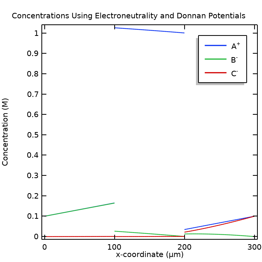
Figure 7. Concentrations when using Donnan potential conditions and electroneutrality.
Further Boosting Model Convergence
There is actually one more simplification of the model problem that can be done: We can assume that the ion-exchange membrane completely blocks all ions but A+. In this case, the concentrations of B– and C– in the membrane are 0, and due to electroneutrality, the concentration of A+ is always constant and given by the immobilized charge. As a result, we do not need to solve for any concentration variable in the membrane. Since there are no concentration gradients of A+ in the membrane, the sole domain equation simplifies to the Laplace equation
where we note that, due to electroneutrality, we have
and that the constant electrolyte conductivity can be calculated from
Although this equation is a simplification for multiple mobile ion systems, it should be noted that it is analytically correct for single-ion conductors, such as Nafion in polymer electrolyte fuel cells, where protons are the sole mobile ions present in the membrane.
The Laplace equation is especially well suited for solving with the finite element or boundary element methods that the COMSOL® software uses in the electrochemistry interfaces. Aside from reducing the degrees of freedom and the corresponding memory requirements of the solver further, the fully blocking membrane assumption facilitates the solver convergence. For example, there is no longer a need for ramping up the fixed ion concentration by using an auxiliary sweep in the stationary solver as I described earlier.
Figure 8 compares the concentration of A+ and potential, respectively, between the NPP (the results when using electroneutrality and Donnan conditions are identical) and the model using a fixed membrane charge. For our example problem, the fully blocking model approximates the original model fairly well.


Figure 8. Comparison of the A+ concentration (left) and potential (right) between the NPP model and the simplified model, assuming a fully blocking membrane.
How to Build an Ion-Exchange Membrane Model in COMSOL Multiphysics®
The Ion-Exchange Membrane domain node in the Tertiary Current Distribution interface can be used to set up the correct domain equations based on the choice of charge conservation model. In the case of electroneutrality, it also sets up the Donnan conditions automatically on boundaries to neighboring electrolyte domains. There is also an Ion Exchange Membrane Boundary node available for setting up Donnan conditions on boundaries between different physics interfaces.
To build the NPP model, we can use one instance of the Tertiary Current Distribution interface with the charge conservation model set to Poisson. We can then use the Electrolyte domains to define the free electrolyte domains, and the Ion Exchange Membrane node to define the membrane domain.
To build the model based on electroneutrality and Donnan conditions, we can proceed as above but switch the charge conservation model to Electroneutrality. This applies the Donnan conditions automatically to the internal boundaries.
Building the fully blocking membrane model requires a few more steps. Since separate concentration variables are solved for on each side of the membrane (A+ and B- on the left; A+ and C- on the right), we have to use two separate instances of the Tertiary Current Distribution interface (with the charge conservation model set to Electroneutrality). We can use a Secondary Current Distribution interface for the membrane to solve for the potential using the Laplace equation and the Ion-Exchange Membrane Boundary nodes in the Tertiary Current Distribution interfaces to set up the Donnan potential conditions.
Next Steps
Download the MPH-file for this model from the Application Gallery:
Read more about modeling electrochemical applications in this blog post: Advancing Vanadium Redox Flow Batteries with Modeling.
Editor’s note: This blog post was updated on 10/25/2018 to include information about new features available as of version 5.4 of COMSOL Multiphysics.
Nafion is a registered trademark of The Chemours Company FC, LLC.


Comments (24)
Zhidong Zhang
September 26, 2018Hi Henrik,
This is a very nice and detailed blog. Have you uploaded the associated files that we can download to learn?
Best,
Zhidong
Henrik Ekström
September 27, 2018Hi Zhidong.
Thanks for your comment. I have a model file prepared for the upcoming 5.4 version. We will make this file available for download as soon as we have released the new version. It should not be too long now.
Henrik
Henrik Ekström
October 26, 2018Hi again Zhidong – we have added a link so that you can download the model mph file now.
Henrik
Yuan Lin
February 7, 2019Hi Henrik,
This blog and the model file demonstrate clearly how the three approaches work and the differences between them, which is very illustrating. Thanks.
Best regards
Yuan
Lasse Murtomäki
March 12, 2019This is exactly what I have been looking for. Thank you. Since when the Ion Exchange Membrane Boundary has been there? I have tried to do my own model but failed miserably.
Henrik Ekström
March 14, 2019Thanks Lasse. We released the Ion Exchange Membrane domain node, with automatic setup of the corresponding boundary condtitions, in the 5.4 release last fall. (We had however a Ion Exchange Membrane Boundary node earlier, but it did not support multiple ions until 5.4).
Lasse Murtomäki
May 15, 2019Hej Henrik
Changing anion B to two-valent (e.g. sulfate) the model does not converge any more.
mvh
Lasse
Lasse Murtomäki
May 15, 2019Fortsätter…
Also, making the total concentrations in the domain limits different crashes the calculation. I also tried a binary solution, but then the problem seems to be over-defined because Comsol nags about degrees of freedom.
mvh
Lasse
Henrik Ekström
May 15, 2019Hi Lasse.
Please contact support if you have problems running the model. (It is easier to help you via support since you can attach your modified model file there.)
Regards
Henrik
Lasse Murtomäki
May 16, 2019Henrik
It is exactly your model, I only changed the charge number or boundary concentrations. Have you tried that?
mvh
Lasse
Lasse Murtomäki
May 16, 2019Hej
Now it works. I do not know why 🙂 Problem solved.
Thanks!
mvh
Lasse
Biswabhusan Dhal
June 22, 2019can I get a 5.3 v of this model
thanks
Kiana Amini
January 20, 2020Running the example file in Comsol version 5.5, returns a warning “No potential condition found. Problem may have infinitely many solutions.
– Node: Secondary Current Distribution (cd)”, but it works in version 5.3. Can you please clarify how I can get rid of the warning?
Henrik Ekström
January 21, 2020 COMSOL EmployeeDear Kiana.
The model works. The warning just indicates that the Secondary Current Distribution interface does not detect any potential constraints within itself. (The potential is implicitly constrained from the Tertiary Current Distribution interfaces.) I am afraid there is no way to get rid of the warning.
Swamenathan Ramesh
April 8, 2022Hello Henrik,
Is it possible to get the COMSOL 5.6 version of this model? I have been trying to build the NPP model on my own but have been unsuccessful. The solution blows up. It would be great to know where I am going wrong and what I am missing.
Thanks and regards
Swamenathan
Henrik Ekström
April 12, 2022 COMSOL EmployeeHi Swamenathan. Please send a messsage to our support and we’ll send you the file.
Swamenathan Ramesh
April 13, 2022Thanks for the reply, I will do that.
Meanwhile, I have been doing the NPP model myself and was able to successfully reproduce figures 4, 5 and 6 (species concentrations, electrolyte potential and electrochemical potential) but am not able to get the molar flux plot. I am using the Fick’s law to define my molar flux variables but the result is erroneous. For example, molar flux of species A remains zero throughout but shoots up to high values at the ion exchange membrane – free electrolyte boundaries. As far as I know, the formula for the molar flux (M_A = -Da*(d(cA,x))) is right where Da is the diffusion coefficient, cA is the concentration of species A and x is the spatial coordinate. Any insights would be appreciated.
Thanks
Swamenathan
Henrik Ekström
April 13, 2022 COMSOL EmployeeThe molar flux, defined by equation 4 above in the blog, also depends on the gradient of the potential.
Swamenathan Ramesh
April 13, 2022Used equation 4 from the blog and am still faced with similar issues. I also realized that I do not know how to plot against the auxiliary sweep parameter (first time COMSOL user) as I get the plot at only point when plotting against c_fix (concentration of immobilized ion) which was globally defined with a value of 1 M. When plotting, this is the value for x-axis being taken instead of auxiliary sweep values of c_fix (range(0,1,1000)). Nevertheless, my flux values are wrong. I am defining it as M_A = -(Da/(R_const*T))*cA*(d(mu_A,x)) where mu_A is the electrochemical potential of A and T is the ambient temperature.
Henrik Ekström
April 14, 2022 COMSOL EmployeePlease contact support for your enquiries, which will also enable you to send your model to us.
hamid hammed
May 7, 2022Hi dear Henrik
I want to model a ceramic membrane in which electrons and ions move simultaneously. Is there a physics in Comsol that can be used? Or should I use the PDE module?
Henrik Ekström
May 9, 2022 COMSOL EmployeeHi Hamid.
I am not sure what would be the best way to do this. It depends on the equations you want to solve for. Possibly there is functionality in the Semiconductor Module you could use. I suggest you contact support.
洪博 郑
October 8, 2023Hello, Teacher Henrik Ekström, regarding the setting of Donnan potential, is it used as a boundary condition? And as a way to describe the relationship between concentration and potential, what role does it play in computational solving? Or is it used to solve concentration variables or potential variables?I would greatly appreciate it if you could provide some insights!
Henrik Ekström
October 13, 2023 COMSOL EmployeeThe Donnan potential conditions are used as a boundary conditions for the dependent variables on the internal boundaries between the ion-exchange membrane and free-electrolyte domains.