
Music blasts from a person’s laptop. A loud and clear DING alerts a smartwatch user to a new text. BEEP, BEEP, BEEP: A cellphone alarm wakes up its owner. Consumers expect great sound quality, no matter the size of their device. As electronics continue to decrease in size, the importance of well-designed microspeakers rises. Simulation software can help you design minimized microspeakers with great sound quality.
Challenges to Designing Microspeakers
With tablets and smartphones, consumers can be tuned in and listening to streaming services, music apps, and podcasts on the go. Further, as of 2019, video accounts for about 78% of the world’s mobile data traffic. People are always going to expect the best sound quality, even when their devices get smaller and more portable. Great sound quality comes from thoroughly planned and well-designed microspeakers.
Microspeakers’ tiny frames make them a challenge to design. Luxuriously loud audio does not come easy for any speaker, especially in one of this size. The delicate diaphragm can even break apart when faced with sound pressure levels (SPLs) that are too extreme, which can lead to a blown speaker. Aside from taking the fragile diaphragm into account, acoustics engineers also need to create a design that avoids voice coil and diaphragm melting caused by excessive current flow.
Using simulation software, engineers can test and improve their microspeaker designs multiple times through the development cycle, greatly reducing the need for physical prototyping and saving time and money in the process. Another advantage of this virtual design loop over traditional physical prototyping and testing is that simulation gives much more insight into what drives the performance of the microspeaker. Simulation models generate an amount of valuable information that would be impossible to obtain with a physical test, as any magnitude can be measured at any location of the model at any frequency.
Below, we compare the characteristics of an Ole Wolff microspeaker with a simulation of the speaker, using the COMSOL Multiphysics® software and add-on Acoustics Module.
Electromagnetic, Mechanical, Vibroacoustic, and Thermoviscous Analyses of a Microspeaker
Model Overview
The OWS-1943-8CP microspeaker is a discontinued microspeaker from Ole Wolff that consists of several different parts, including:
- Diaphragm
- Voice coil
- Magnet
- Pole piece
- Front plate
- Back vents
Due to its size, a microspeaker’s layout varies compared to a traditional loudspeaker. For instance, the diaphragm often functions as both a dust cap and a spider. They are also extremely small: The dimensions of the microspeaker modeled here are about 19 mm in diameter and 2.8 mm in height, making it smaller than a U.S. penny!


The OWS-1943T-8CP microspeaker, with its front plate from top and bottom views. The geometry is copyright by Ole Wolff Elektronik A/S.
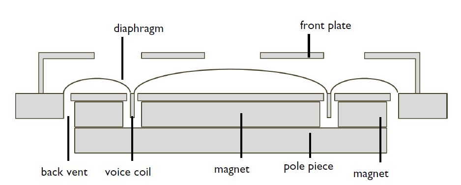
Schematic cross-section view of the microspeaker.
Electromagnetic Analysis
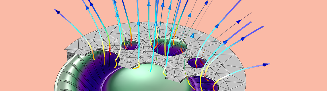
Most microspeakers use a permanent magnet to create a magnetic field surrounding the voice coil. When an audio signal is applied as an alternating current to the voice coil, due to Faraday’s law of induction, an electromagnetic force is generated in the voice coil. This alternating force makes the diaphragm vibrate in the axis of the speaker, generating pressure waves that propagate to the surrounds and thus generate sound. The response of the microspeaker for a given audio signal will be a combination of the electromagnetic, mechanical, vibrational, and acoustic properties of the microspeaker, making COMSOL Multiphysics naturally suited to analyze this highly coupled multiphysics problem. The first logical step is to analyze the electromagnetic circuit, which generates the force that excites the vibrations of the diaphragm.
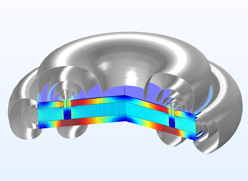
Electromagnetic analysis of the speaker motor showing the model’s magnetic flux density. Saturated areas are shown in red.
With the electromagnetic analysis, we can gain insight into the performance of the speaker; knowing, for example, if magnetic saturation is reached at the pole piece; identifying eddy currents induced due to the current going through the voice coil; or identifying how the induction force over the voice coil changes as the voice coil moves along the axis of the speaker (one parameter of interest being BL(x)), which influences how the speaker will distort the acoustic signal when large signals are applied.
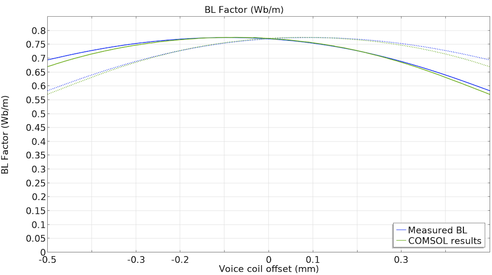
BL factor as a function of coil displacement; BL(x).
Mechanical Analysis
Ideally, the compliance (inverse of the stiffness) of the diaphragm should be constant, as the diaphragm moves away or closer to the magnet. When large acoustic signals are applied to the speaker and this displacement becomes large enough, the variation of compliance (also known as CMS(x)) or nonlinearity can induce distortion on the acoustic signal. To assess this, we will make use of the nonlinear analysis capabilities of COMSOL Multiphysics and analyze how the geometric nonlinearities will affect the stiffness of the diaphragm.
To test the accuracy of the model, we can perform a comparison between the physical measurements and the measurements predicted by the model. This comparison is usually referred to as correlation, and it is quite commonly used at different stages to gain confidence on the validity of the model. In the graph below, you can see a good match between the model and the measurements for positive voice coil displacements (when the diaphragm moves away from the magnet).
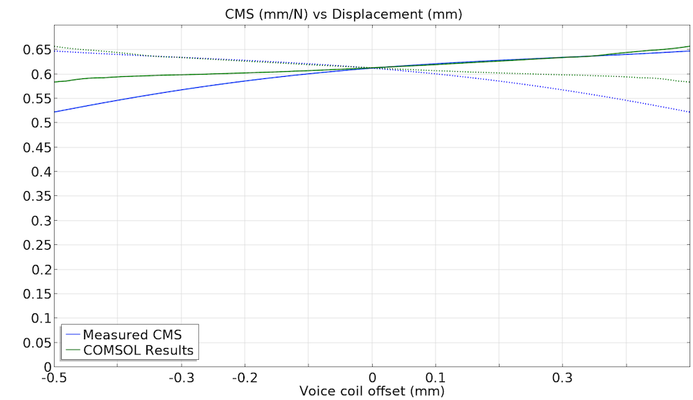
Measured compliance of the Ole Wolff microspeaker (blue) and COMSOL Multiphysics model (green).
Vibroacoustic Analysis
Once the electromagnetic characteristics of the system are known, it is possible to perform a vibroacoustic analysis of the microspeaker for small acoustic signals. In this analysis, the electromagnetic force generated on the voice coil is countered by the inertial forces, the mechanical forces generated by the diaphragm, and the pressure force created by the air.
The coupled structural and acoustic response, or vibroacoustic response, will modify how the current going through the voice coil translates into the SPL at a certain location. Of the physical measurements available from the test, one of the most direct measurements to compare is the total impedance of the speaker. The impedance is a measurement of the opposition that the voice coil presents to a current when a voltage is applied and it has a strong dependency of the frequency at which this voltage is applied.
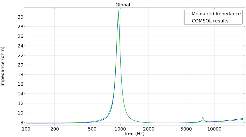
Measured impedance of the Ole Wolff microspeaker (blue) and COMSOL Multiphysics model (green).
In the graph above, you can see the main peak at 950 Hz, where the impedance for the model and the physical microspeaker match almost perfectly. This peak is known as resonant frequency, and it is the frequency below which a loudspeaker is increasingly unable to generate sound output for a given input signal. The resonant frequency is also the first vibroacoustic mode of the speaker, which relates to how stiff the diaphragm is and the total mass of the voice coil. There is also a smaller peak around 7300 Hz, which is caused by the interaction between the back cavity and a radial mode. For this peak, the model is underpredicting the damping, showing a narrower peak. The reason for this is that the thermoviscous losses in the back cavity are quite relevant, as will be discussed later. Even with this minor disparity in results, the simulation still proves to have high levels of agreement with the physical model.
The simulation model’s voice coil and diaphragm functioning as a piston at 1000 Hz (left), and the distortion of its diaphragm and voice coil at 11,200 Hz (right).
Another relevant piece of information that can be obtained from the vibroacoustic analysis is the deformation/movement of the diaphragm as the frequency increases. At a low frequency, the diaphragm will show a deformation where most of the central part of the diaphragm is working as a rigid piston, pushing air as it travels back and forth. As the frequency increases, higher-order modes could be excited, making the diaphragm less effective and thus reducing the sound projected by the microspeaker. This phenomenon is known as diaphragm breakup and it is one of the main drivers used to design the shape and material of the diaphragm. In the animations above, you can see the displacement in a color map for two frequencies. The image on the left shows the model’s diaphragm and voice coil functioning close to an ideal piston at 1000 Hz, while the image on the right shows the distortion at 11,200 Hz, where the center of the diaphragm and the voice coil do not act as a rigid body anymore.
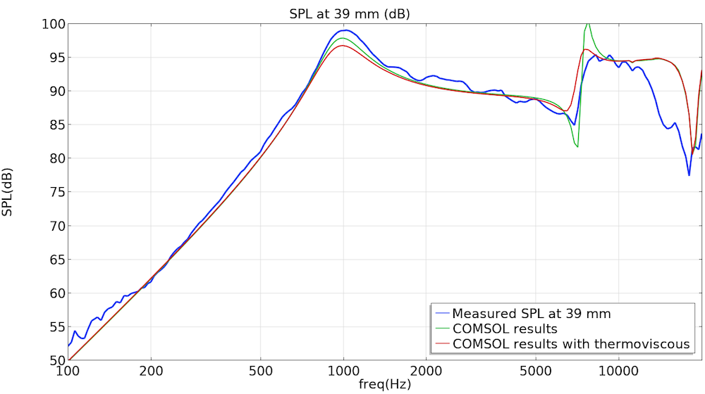
Measured SPLs of the physical microspeaker at 39 mm (blue), the COMSOL Multiphysics results (green), and the COMSOL Multiphysics results with thermoviscous analysis included (red).
The SPL evaluated 39 mm in front of the microspeaker is also a good metric to check the accuracy of the model. This is known as the response of the speaker. As shown in the picture above, the model shows a very good level of correlation from low frequencies up to 5000 Hz. The difference between the model and the measurements around 7300 Hz indicate that the model is underpredicting the damping, and that is likely related to the thermoviscous losses, which are not considered in the tutorial model (green curve).
Thermoviscous Analysis
Thermoviscous effects are important to pay attention to, especially when designing microspeakers. Sound waves become weaker after they spread in small structures due to thermal and viscous losses in the acoustic boundary layers.
In order to get results that more closely relate to the physical microspeaker’s SPL, another study can be run using COMSOL Multiphysics, considering the thermoviscous acoustic properties of the back cavity. In the graph above (red curve), you can see that the COMSOL Multiphysics results, when including thermoviscous acoustics, are a much better match to the physical microspeaker’s results. Thermoviscous modeling is a very powerful and predictive way to assess the losses in small electronic equipment, but this precision usually comes with a longer computing time.
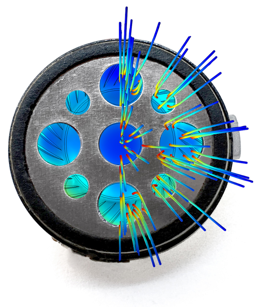
The Ole Wolff microspeaker with the model superimposed.
In this blog post, we have demonstrated a possible method to analyze a model from an industry example and how this analysis can lead to meaningful results that drive the design process. When working with complex models, it is good practice to perform correlations to measurements at different stages of increasing complexity. A high level of correlation can be achieved using COMSOL Multiphysics based on the geometry of the speaker and a set of relatively simple assumptions. Correlation can be used to understand what parts of the model show a good level of accuracy and what parts may need a more detailed modeling approach. COMSOL Multiphysics is an established software to analyze industrial applications and produce accurate predictions for different levels of model complexities.
Next Steps
Try modeling this industry-scale microspeaker model yourself, and analyze a variety of important multiphysics characteristics, by clicking the button below. Doing so will take you to the Application Gallery example.

Comments (0)