Copying and Reusing Boundary Mode Analysis Results
When using the Beam Envelopes or the Electromagnetic Waves, Frequency Domain interfaces in COMSOL Multiphysics®, one can often have multiple Port boundary conditions that have identical structures but are at different locations in space. It is often the case, especially for optical and photonics models, that multiple different modes at these ports are of interest, and these modes need to be numerically computed. It is possible to compute all of the modes of interest using just a single Port boundary condition of type Numeric and to copy and reuse these solutions in all of the other ports in the model, which will be User-Defined Ports.
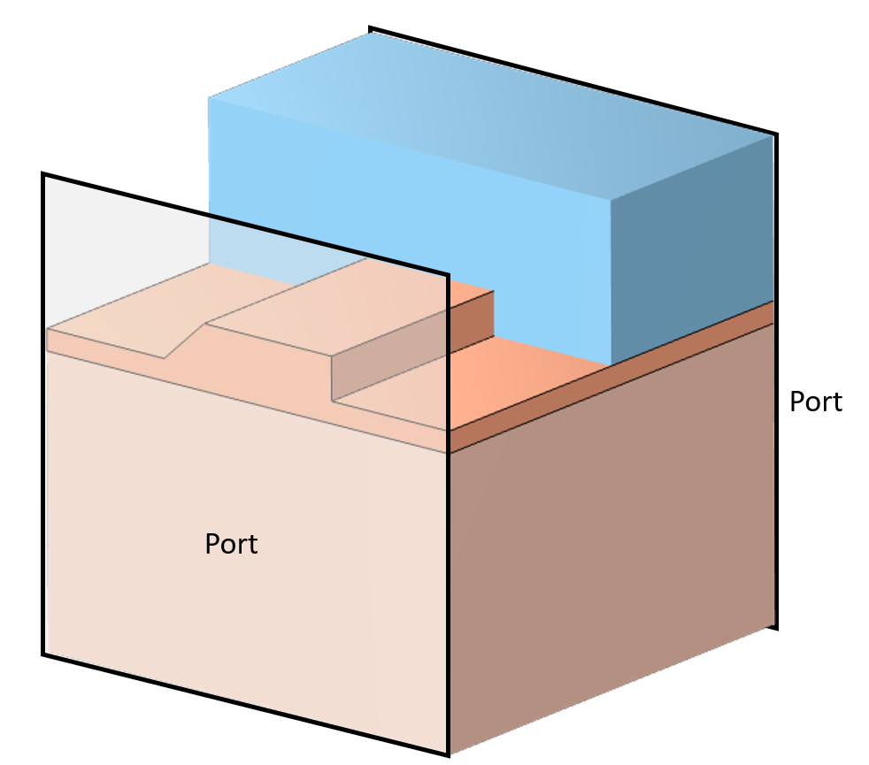
A supporting example is shown below: an optical ridge waveguide that does not change shape along the length. A mode of a particular polarization is launched, but other modes can exist due to anisotropic properties that exist in part of the substrate. For this example, the first two modes of propagation are considered.
Precomputing All of the Modes of the Waveguide
This technique begins with first defining a Numeric Port that will be used to compute all of the modes of interest. Since the Port will not be used directly in the ultimate analysis, give it a Port number of 0 to clearly differentiate it. Apply the Port boundary condition to the boundaries describing the waveguide. For optical waveguides, ensure that the width of the cladding region is large enough that the fields fall off to nearly zero.
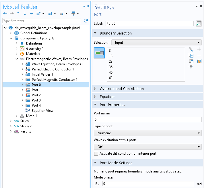
Setting up a single Numeric Port.
Set up a study containing a boundary mode analysis that solves the modes of this Port. In this example, only the first two modes are of interest, so set the Desired number of modes to 2, and set the Search for modes around shift setting to an effective mode index of 3.5, which is the highest refractive index in the waveguiding structure. This will compute the first two modes supported by this waveguiding structure at this frequency.
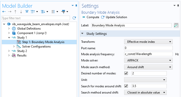
Solver settings for computing all of the modes of interest.
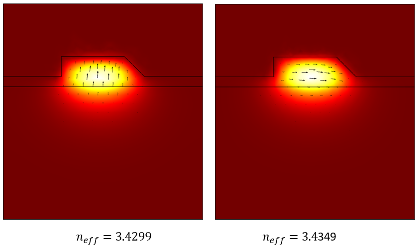
Once the study is solved, it is helpful to create plots of the boundary mode electric field to verify the computed modes. It is these fields that will be used in the next step to define a set of user-defined ports.
Understanding and Using the Outputs of the Boundary Mode Analysis
The total boundary mode electric field is composed of two orthogonal components, the electric field tangent to the boundary and the electric field normal to the boundary. The total electric field is:
 ,
,
where the tangent component of the field is a vector that lies in the plane of the boundary, and the normal component is a scalar field. The normal vector,  , is the vector pointing outward from the modeling domain; it points in the direction of an outgoing signal.
For port index 0, the components of the tangential field are: ewbe.tEbm0x, ewbe.tEbm0y, and ewbe.tEbm0z, and the normal component is ewbe.nebm0. The components of the outward normal vector are ewbe.nx, ewbe.ny, and ewbe.nz, and so the total electric field of the mode on that boundary is:
ewbe.tEbm0x-ewbe.nx*ewbe.nebm0
ewbe.tEbm0y-ewbe.ny*ewbe.nebm0
ewbe.tEbm0z-ewbe.nz*ewbe.nebm0
Each of the two computed modes of Port 0 will have a different tangential and normal component, as well as a propagation constant: ewbe.beta_0. To refer to these variables, use the withsol operator, which has the following syntax: withsol('sol1',Ex_total, setind(lambda,M1)).
The first argument is the solution tag, so any solution can be referred to. (See also: Examples of the withsol Operator.) The second argument is the expression to evaluate from that solution, and the third argument uses the setind operator, which here uses one of two parameters, M1=1, M2=2, to refer to the two modes computed by the Boundary Mode Analysis study. This operator allows for the reuse of these precomputed solutions.
Next, the fields computed on Port 0 have to be mapped to the other boundaries where they will be needed. This is done via the General Extrusion operator with settings as shown in the screenshot below. The input and output ports are at identical xy-coordinates, so no change to the mapping of these is needed. The z-expression of z-Length is used here because the output boundaries are offset in the z direction by the Global Parameter, Length. This operator will make the data computed on the input boundaries available on the output boundaries. For full details on using the General Extrusion operator, including for rotating the fields, see: Examples of the General Extrusion Operator.
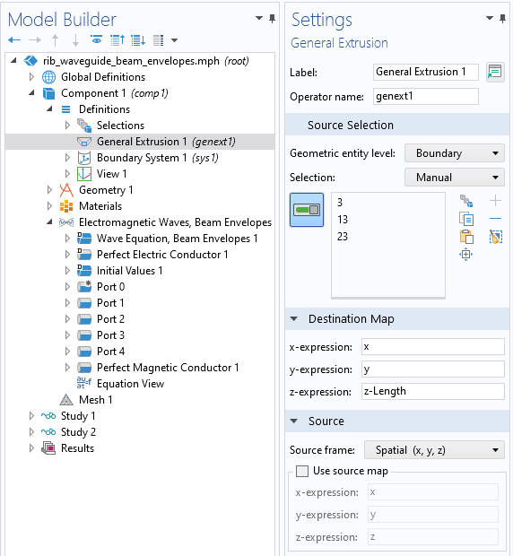
The settings for the General Extrusion operator, which maps data from one boundary to another. Note the Variables nodes under Definitions_, where the_ withsol and General Extrusion operators are used to define the mode fields and propagation constants for Port 1 to Port 4.
To use this operator, which has the default name genext1, at the other port boundaries, wrap the previously developed expressions with the genext1() operator. So, for example, the total electric field of the first mode, mapped to the outgoing port, is of the form:
genext1(withsol('sol1',ewbe.tEbm0x,setind(lambda,M1)))-ewbe.nx*genext1(withsol('sol1',ewbe.nebm0,setind(lambda,M1)))
genext1(withsol('sol1',ewbe.tEbm0y,setind(lambda,M1)))-ewbe.ny*genext1(withsol('sol1',ewbe.nebm0,setind(lambda,M1)))
genext1(withsol('sol1',ewbe.tEbm0z,setind(lambda,M1)))-ewbe.nz*genext1(withsol('sol1',ewbe.nebm0,setind(lambda,M1)))
Note that the General Extrusion operator is not applied to the components of the normal vector since this has different components on opposite boundaries. In practice, a set of variables can be created to simplify this syntax.
Using the Precomputed Modes and Setting up the Model
To define the waveguide model where all Ports are using these precomputed mode fields, begin by defining the excitation port, Port 1, on the same set of boundaries where Port 0 was defined. Set the Type of port to User defined and, within the Port Mode Settings section, use the previously defined variables that refer to the total electric field and propagation constant at each of the four ports.
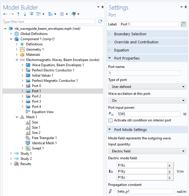
Settings for a port to reuse previously computed electric fields and propagation constants that exist at the same boundaries.
Repeat the abovementioned steps and define Port 2 on the same set of boundaries. This is an unexcited port that will monitor reflections back into the second mode. Set the wave excitation off, and use the variables P2Ex, P2Ey, and P2Ez for Electric mode field and beta_p2 for Propagation constant. Also define two more ports for the outgoing signal on the far side.
It is a requirement that the meshes on all Port boundaries are identical, and this condition can be satisfied in general via the Identical Mesh feature, as shown in the screenshot below.
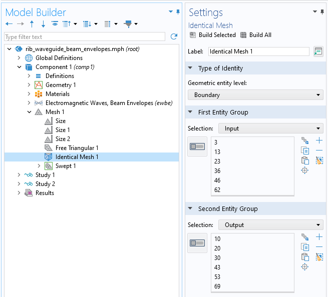
Using the Identical Mesh feature to ensure that the mesh on the input and output ports are identical.
In regard to meshing for this particular case, the mesh must be sufficiently refined both in the cross-sectional plane and along the length. Since the supported modes in the anisotropic substrate region are slightly different from the isotropic substrate region, the mesh refinement along the length must be studied. For further guidance on meshing and solving such models, see the Directional Coupler model.
When solving, an optional Study Reference can be used to recompute the Port 0 modes before solving the 3D model. In the Wavelength Domain study step, disable Port 0 within the Physics and Variables Selection section, as shown below.
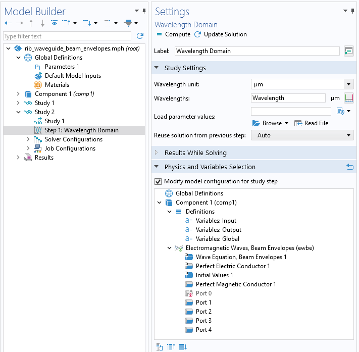
Visible in the Settings window, Port 0 is disabled when computing the fields within the model.
Submit feedback about this page or contact support here.