CFD Module

Simulate Single-Phase and Multiphase Flow

Perform computational fluid dynamic simulations with the CFD Module, an add-on product to the COMSOL Multiphysics® software. The CFD Module provides tools for modeling the cornerstones of fluid flow analyses, including:

  • Internal and external flows
  • Incompressible and compressible flows
  • Laminar and turbulent flows
  • Single-phase and multiphase flows
  • Free and porous media flows

The multiphysics capabilities are virtually unlimited within the module and in combination with other add-on modules to COMSOL Multiphysics®. The CFD Module provides you with the tools to model nonisothermal flow with conjugate heat transfer, reacting flow, fluid–structure interaction (FSI), and electrohydrodynamics (EHD). Additional multiphysics couplings can be added together with other modules from the COMSOL product suite, such as combining fluid flow with large structural deformations in FSI. The simulation environment looks the same regardless of what you are modeling.

Contact COMSOL
A model of a sports car with two side mirrors and two doors with yellow streamlines showing the flow field from the front to the rear of the car.

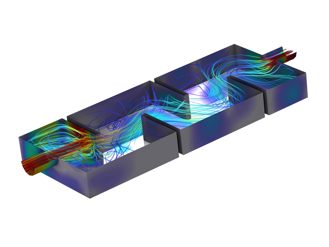
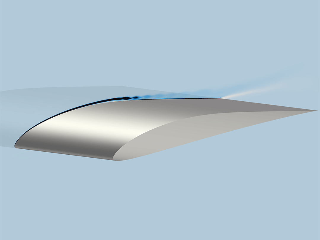
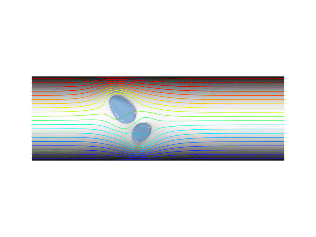
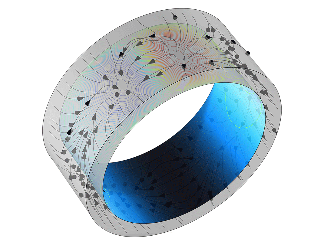
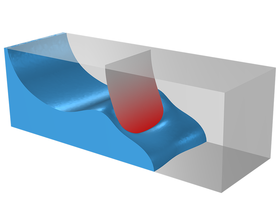
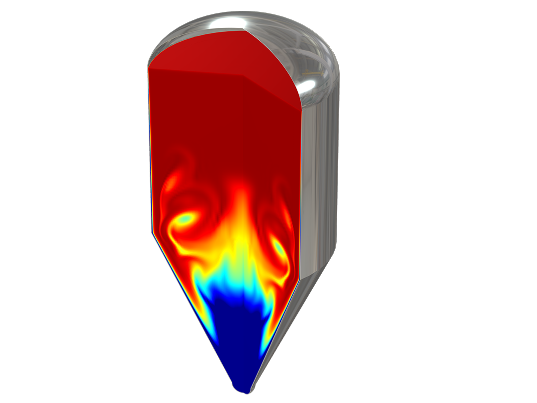
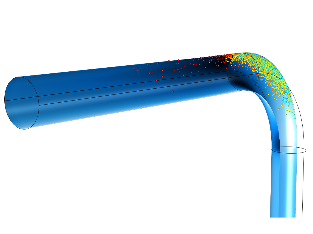
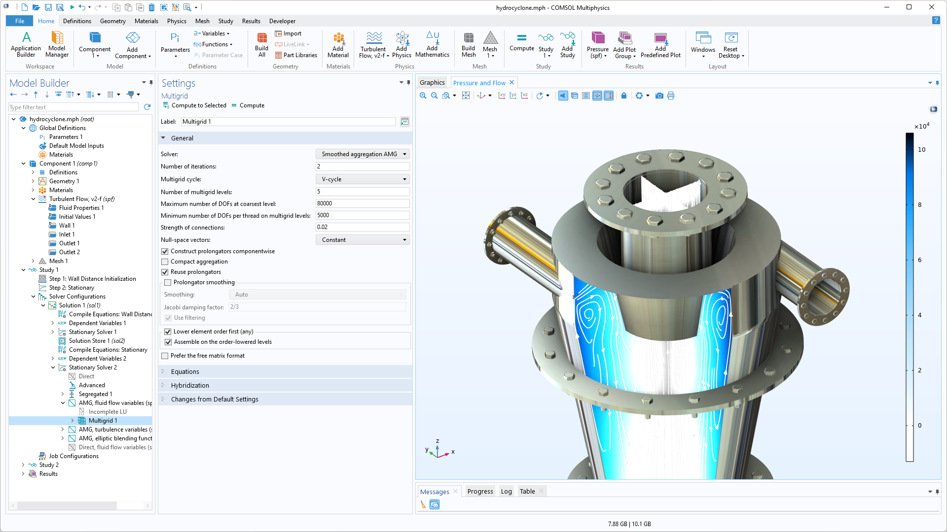
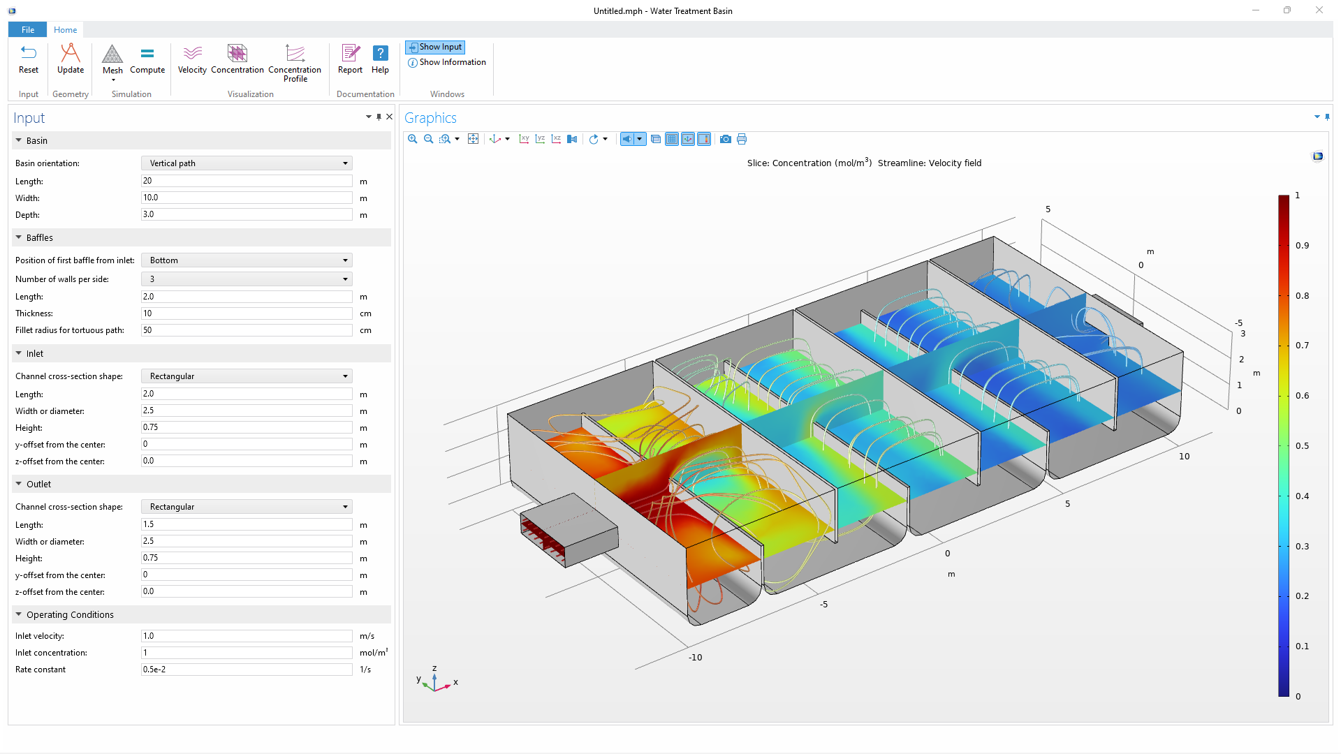
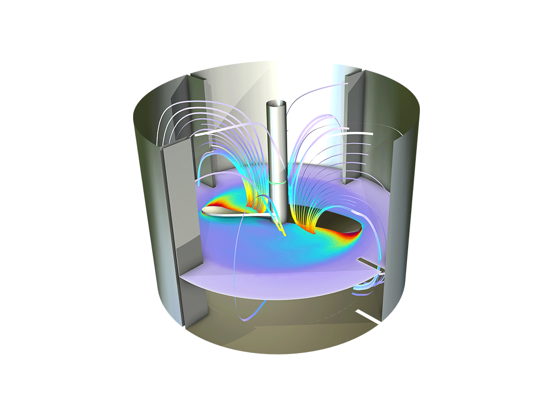
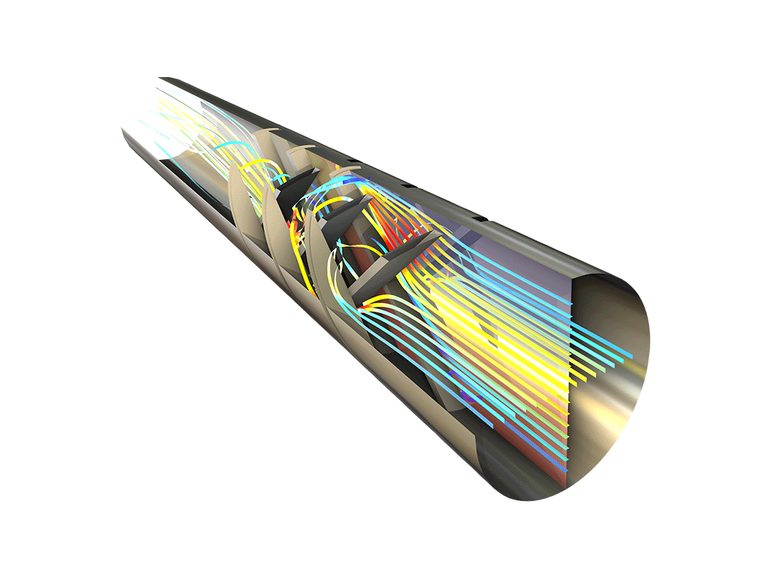
Laminar and Creeping Flow

Model transient and steady laminar flow with the Navier–Stokes equations or creeping flow with the Stokes equations.

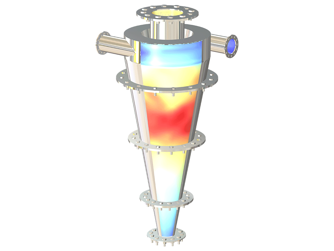
In addition to modeling fluids with constant density and viscosity, you can study fluids where the viscosity and density depend on the temperature, local composition, electric field, or any other modeled field or variable. In general, density, viscosity, and momentum sources can be arbitrary functions of any dependent variable, as well as derivatives of dependent variables.

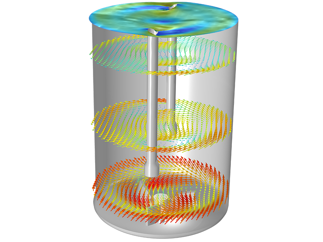
For non-Newtonian fluids, you can use the generic yet predefined rheology models for viscosity, such as Power Law, Carreau, Bingham, Herschel–Bulkley or Casson for easy model setup.

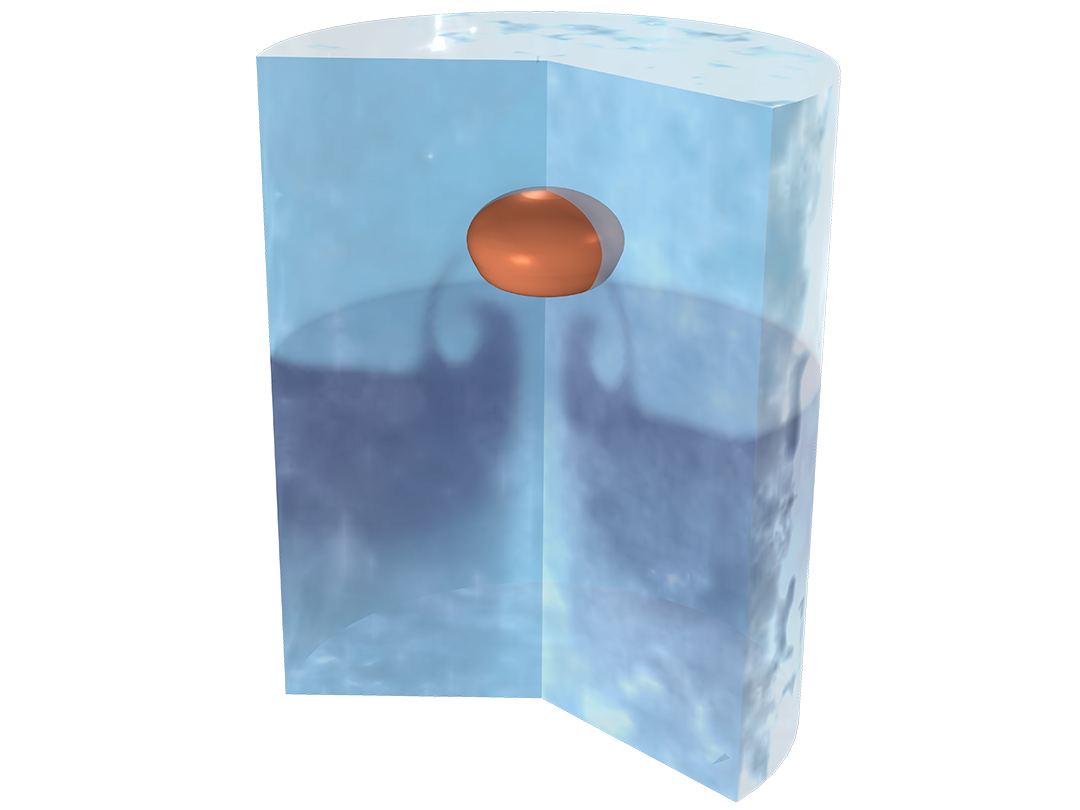
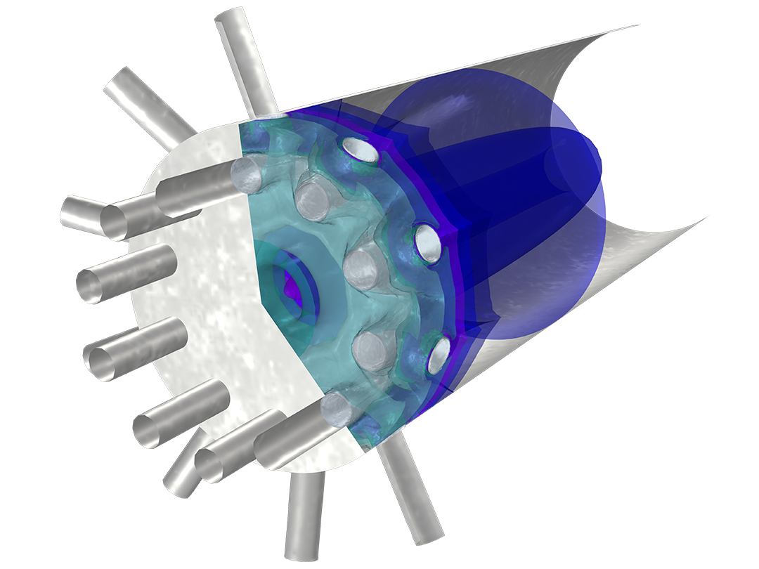
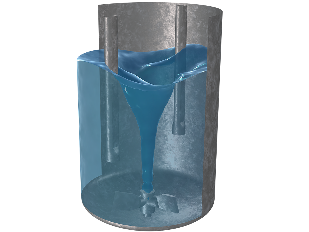
You can also model laminar flow in moving structures, for example opening and closing valves or rotating impellers.

Turbulent Flow

A comprehensive set of Reynolds-averaged Navier–Stokes (RANS) turbulence models are available in predefined flow interfaces in the CFD Module. These models allow you to simulate a wide range of steady and transient turbulent flows. You can also change or extend the model equations directly in the user interface to create turbulence models that are not yet included.

RANS Turbulence Models

Two-Equation Models
  • k-ε
  • Realizable k-ε
  • k-ω
  • SST
  • Low-Re k-ε
Additional Transport Equation Models
  • Spalart–Allmaras
  • v2-f
Algebraic Turbulence Models
  • Algebraic yPlus
  • L-VEL

Wall Treatment

A detailed view of the wall resolution and velocity flow of a water treatment basin model.
Wall Functions

Robust and applicable for coarse meshes, with limited accuracy.

A close-up view of an Eppler 387 model showing the boundary-layer transition.
Low-Reynolds-Number Treatment

Resolves the flow all the way down to the walls. Accurate but requires a fine mesh.

A detailed view of a hydrocyclone model showing the fluid velocity.
Automatic Wall Treatment

Inherits the robustness provided by wall functions, with an accuracy of low-Re treatment in well-resolved regions.

Large Eddy Simulation (LES)

Large eddy simulation (LES) is used for resolving larger three-dimensional unsteady turbulent eddies, whereas the effects of the smaller eddies are approximately represented. When combined with boundary layer meshing, this technique gives an accurate description of a transient flow field as well as accurate fluxes and forces at the boundaries. The LES models — residual-based variational multiscale (RBVM), residual-based variational multiscale with viscosity (RBVMWV), and Smagorinsky — are applicable to incompressible and compressible flows.

Detached Eddy Simulation (DES)

Detached eddy simulation (DES) combines RANS and large eddy simulation (LES), where RANS is used in the boundary layers and LES is used elsewhere. DES combines the Spalart–Allmaras turbulence model with the LES models: RBVM, RBVMWV, or Smagorinsky. The wall treatment for Spalart–Allmaras is either a low Reynolds number or an automatic wall treatment.

The benefit of DES is that it requires a less dense boundary layer mesh than a pure LES. This substantially reduces the memory requirements and computation time when the model equations are being solved. The DES models are applicable to 3D, time-dependent, incompressible single-phase flows.

Multiphase Flow and Free Surfaces

In separated multiphase flow systems, you can use surface tracking methods to model and simulate the behavior of bubbles and droplets, as well as free surfaces. For such cases, by using the level set and phase field methods, the shape of the phase boundary can be described in detail, including surface tension effects and topology changes.

When bubbles, droplets, or particles are small compared to the computational domain and there is a large number of them, you can use dispersed multiphase flow models. These models keep track of the mass or volume fractions of the different phases and the influence that the dispersed bubbles, droplets, or particles have on the transfer of momentum in the fluid in an averaged sense. The flow models available are: the bubbly flow, mixture, Euler–Euler, and phase transport mixture models.

Porous Media Flow

The CFD Module makes it simple to simulate fluid flow in porous media using three different porous media flow models. The Darcy's Law model is a robust and computationally inexpensive description of flows in porous structures. It is also available for multiphase flow. The Brinkman Equations model is an extension of Darcy's law that accounts for the dissipation of kinetic energy by viscous shear, and can include inertial effects. Relevant for highly open structures with high porosity, this model is more general than Darcy's law, but also more computationally expensive.

The Free and Porous Media Flow, Brinkman and Free and Porous Media Flow, Darcy models couple flow in porous domains with laminar or turbulent flow (Brinkman) in free domains. The models formulate the Brinkman or Darcy's law equations for the porous domain and the Navier–Stokes equations for the free domains. Turbulent flow in porous media can be simulated in the Brinkman version with any of the epsilon- or omega-based RANS models with additional contributions according to Pedras–de Lemos or Nakayama–Kuwahara, or a combination thereof.

For more details on specific features and functionality, see the Porous Media Flow Module or Subsurface Flow Module.

High-Mach-Number Flow

Model transonic and supersonic flows of compressible fluids in both laminar and turbulent regimes. The laminar flow model is typically used for low-pressure systems and it automatically defines the equations for momentum, mass, and energy balances for ideal gases. High-Mach-number flow is also available for all RANS-equation turbulence models.

In both cases, when solving these models, automatic mesh refinement can be used to resolve the shock pattern by refining the mesh in regions with very high velocity and pressure gradients.

Fluid Flow in Rotating Machinery

Rotating machines, such as mixers and pumps, are common in processes and equipment where fluid flow occurs. The CFD Module provides rotating machinery interfaces that formulate the fluid flow equations in rotating frames, available for both laminar and turbulent flow. You can solve problems using either a full time-dependent description of the rotating system or an averaged approach based on the frozen rotor approximation. The frozen rotor approach is computationally inexpensive and can be used to estimate averaged velocities, pressure changes, mixing levels, averaged temperature and concentration distributions, and more.

Generally speaking, the CFD Module can also solve fluid flow problems on any moving frame, not just on rotating frames, for example opening and closing valves. You can use moving frames to solve a problem where a structure slides in relation to another structure with fluid flow in between, which is easy to set up and solve by employing a moving mesh.

Thin Film Flow

To describe flows in thin domains, such as thin oil films between moving mechanical parts (tribology) or fractured structures, the CFD Module provides the Thin Film Flow interfaces. This formulation is typically used for modeling lubrication, elastohydrodynamics, or effects of fluid damping between moving parts due to the presence of gases or liquids (for example, in MEMS). The predefined Thin-Film and Porous Media Flow coupling can be used to model self-lubrication and squeeze-film flows.

Shallow Water Equations

The shallow water equations allow you to model flow below a free surface under the condition that the horizontal length scale is much greater than the vertical length scale. The shallow water equations are obtained by depth-averaging the Navier–Stokes equations. The dependent variables are the water depth and momentum flux. The equations can be used to model effects of tsunamis and flooding.

Creating Real-World Multiphysics Models

Modeling multiple physics phenomena in COMSOL Multiphysics® is no different than a single-physics problem.

A detailed view of the air flow and temperature of a heat sink model.

Laminar Nonisothermal Flow

Temperature-dependent fluid properties and buoyancy forces; continuous temperature and heat flux across the solid–fluid boundary.

A detailed view of the smoke produced by an incense stick at three different times.

Turbulent Nonisothermal Flow

Low-Re formulation or thermal wall functions for the conjugate heat transfer at solid–fluid boundaries with RANS or LES.

A detailed view of velocity field and deformation of a solar panel model.

FSI: One-Way Studies

Fluid–structure interaction where the flow creates a load on a structure but the deformations are so small that they do not impact the flow.

A detailed view of the fluid–structure interaction of water in a container.

FSI: Fully Coupled1

Fluid–structure interaction where the flow creates loads on a structure, and the deformations are large and affect the flow.

A detailed view of a tank showing the fermentation of beer.

General Reacting Flow

Multicomponent transport and reactions in diluted and concentrated mixtures, using the mixture-averaged model or Fick's law.

A detailed view of a multijet tubular reactor showing the isoconentration surfaces.

Advanced Reacting Flow2

The full Maxwell–Stefan multicomponent transport equations for laminar flows.

A close-up view of a nozzle model with contours.

High-Mach-Number Reacting Flow2

High-Mach-number flow with chemical species transport and reactions for concentrated and diluted species.

A detailed view of a mixer model showing the flow field.

Mixers3

Multiphase flow and free surfaces for rotating machinery, as well as a Part Library for impellers and vessels.

A detailed view of a pipe elbow model showing the velocity as particles.

Particle Tracing4

Euler–Lagrange multiphase flow models, where particles or droplets are modeled as discrete entities.

A detailed view of a heat exchanger pipe model showing the pressure and velocity.

Pipe Flow and CFD5

Pipes and channels connected to 2D or 3D fluid domains with nonisothermal flows, for both laminar and turbulent flows.

  1. Requires the Structural Mechanics Module, MEMS Module, or Multibody Dynamics Module
  2. Requires the Chemical Reaction Engineering Module, Battery Design Module, or Fuel Cell & Electrolyzer Module
  3. Requires the Mixer Module
  4. Requires the Particle Tracing Module
  5. Requires the Pipe Flow Module

General Functionality Adapted for Solving CFD Problems

The CFD Module offers specialized functionality for fluid flow simulations and works seamlessly in the COMSOL Multiphysics® platform for a consistent model-building workflow.

A close-up view of the Model Builder with the Fluid-Structure Interaction node highlighted and a bimetallic strip model shown in the Graphics window.

The Fluid Flow Interfaces

In order to model laminar, turbulent, multiphase, compressible, high Mach number, and thin film flows, as well as the shallow water equations, the CFD Module provides a large number of fluid flow interfaces specialized for different regimes of these flows. Each fluid flow interface defines sets of domain equations, boundary conditions, initial conditions, predefined meshes, predefined studies with solver settings for steady and transient analyses, as well as predefined plots and derived values.

A close-up view of the Mixture Property settings window and an engine gasket model in the Graphics window.

Materials

The CFD Module includes a material library with the most common gases and liquids. In combination with the Chemical Reaction Engineering Module or the Liquid & Gas Properties Module, you can also access generic descriptions for thermodynamic properties of fluids (such as viscosity, density, diffusivity, thermal conductivity, heat of formation, and phase transformation).

A close-up view of the High Mach Number Flow Laminar Settings window, and an Euler bump model shown in the Graphics window

Discretization

The fluid flow interfaces use Galerkin/least-square and Petrov–Galerkin methods to discretize the flow equations and generate the numerical model in space (2D, 2D axisymmetry, and 3D). The test functions are designed to stabilize the hyperbolic terms and the pressure term in the transport equations. Shock-capturing techniques further reduce spurious oscillations. Additionally, discontinuous Galerkin formulations are used to conserve momentum, mass, and energy over internal and external boundaries.

A close-up view of a 1D drag plot and a soccer ball model in the Graphics window.

Evaluating and Visualizing Results

The fluid flow interfaces generate a number of default plots to analyze the velocity and pressure fields. Streamline plots are available to visualize flow and flow direction. Surface and volume plots can be used to show pressure and the velocity vector's magnitude. There is also an extensive list of derived values and variables that can be easily accessed to extract analytical results, for example the drag coefficient.

A close-up view of the Model Builder with the Geometry node highlighted and an ahmed body model shown in the Graphics window.

Geometry

Generate flow domains, such as a bounding box, around imported CAD geometries. Additionally, tools are available to automatically or manually remove details that may not be relevant for fluid flow. With the CAD Import Module, you are able to import most CAD file formats and perform repair and defeaturing operations. The built-in geometry tools for CAD are also able to create complex geometries and domains.

A close-up view of the Mesh Statistics window and a sports car model in the Graphics window.

Meshing

The physics-controlled mesh functionality in the CFD Module takes the boundary conditions in the fluid flow problem into consideration when generating the mesh sequence. A boundary layer mesh is automatically generated in order to resolve the gradients in velocity that usually arise at the surfaces where wall conditions are applied.

A close-up view of the Model Builder with the Multigrid node highlighted and a hydrocyclone model shown in the Graphics window.

Solvers

The flow equations are usually highly nonlinear. To solve the numerical model equations, the automatic solver settings select a suitable damped Newton method. For large problems, the linear iterations in the Newton method are accelerated by state-of-the-art algebraic multigrid or geometric multigrid methods specifically designed for transport problems.

For transient problems, time-stepping techniques with automatic time stepping and automatic polynomial orders are used to resolve the velocity and pressure fields with the highest possible accuracy, in combination with the aforementioned nonlinear solvers.

A close-up view of the input settings of a simulation application and a water treatment basin model in the Graphics window.

Simulation Applications

You can build user interfaces on top of any existing model using the Application Builder, which is included in COMSOL Multiphysics®. This tool enables you to create applications for very specific purposes with well-defined inputs and outputs. Applications can be used for many different purposes: automate difficult and repetitive tasks, create and update reports, provide user-friendly interfaces for nonexperts, increase access to models within your organization, and gain a competitive edge with your customers.

Every business and every simulation need is different.

In order to fully evaluate whether or not the COMSOL Multiphysics® software will meet your requirements, you need to contact us. By talking to one of our sales representatives, you will get personalized recommendations and fully documented examples to help you get the most out of your evaluation and guide you to choose the best license option to suit your needs.

Just click on the "Contact COMSOL" button, fill in your contact details and any specific comments or questions, and submit. You will receive a response from a sales representative within one business day.

Next Step

Request a Software Demonstration