What Is Mass Transfer?
Understanding Mass Transfer
Mass transfer describes the transport of mass from one point to another and is one of the main pillars in the subject of Transport Phenomena. Mass transfer may take place in a single phase or over phase boundaries in multiphase systems. In the vast majority of engineering problems, mass transfer involves at least one fluid phase (gas or liquid), although it may also be described in solid-phase materials.
In many cases, the mass transfer of species takes place together with chemical reactions. This implies that flux of a chemical species does not have to be conserved in a volume element, since chemical species may be produced or consumed in such an element. The chemical reactions are sources or sinks in such flux balances.
The theory of mass transfer allows for the computation of mass flux in a system and the distribution of the mass of different species over time and space in such a system, also when chemical reactions are present. The purpose of such computations is to understand, and possibly design or control, such a system.
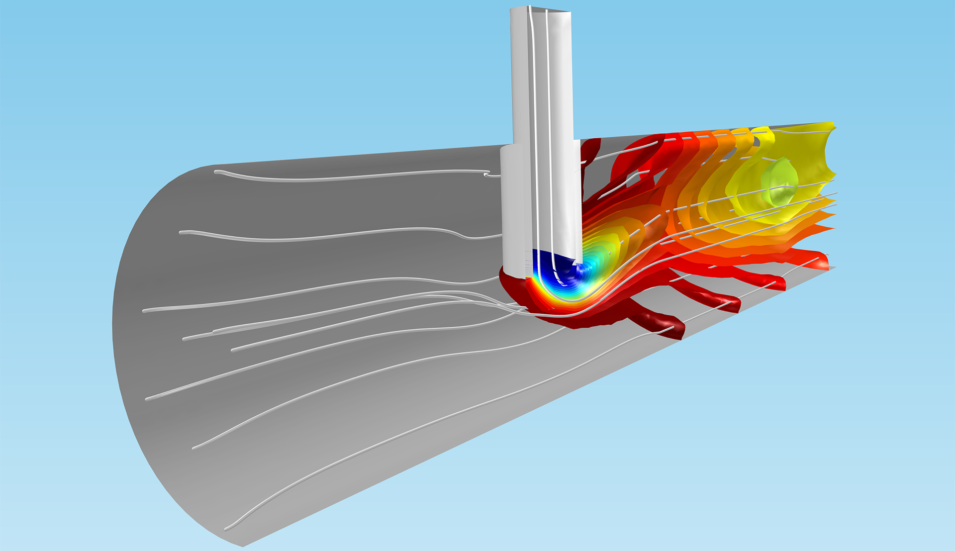 Transport and reactions in a reactor. The concentration isosurfaces reveal mass transfer through diffusion and convection. The flux through diffusion takes place perpendicular to the concentration isosurfaces, i.e., the reactions may cause a flux to the reaction site of the species that are consumed in the reaction. Convection creates a larger separation between the concentration isosurfaces and takes place along the streamlines of the fluid flow (in white), which in some places run along the isosurfaces, since convection tends to eliminate concentration gradients along its main direction.
Transport and reactions in a reactor. The concentration isosurfaces reveal mass transfer through diffusion and convection. The flux through diffusion takes place perpendicular to the concentration isosurfaces, i.e., the reactions may cause a flux to the reaction site of the species that are consumed in the reaction. Convection creates a larger separation between the concentration isosurfaces and takes place along the streamlines of the fluid flow (in white), which in some places run along the isosurfaces, since convection tends to eliminate concentration gradients along its main direction.
Transport and reactions in a reactor. The concentration isosurfaces reveal mass transfer through diffusion and convection. The flux through diffusion takes place perpendicular to the concentration isosurfaces, i.e., the reactions may cause a flux to the reaction site of the species that are consumed in the reaction. Convection creates a larger separation between the concentration isosurfaces and takes place along the streamlines of the fluid flow (in white), which in some places run along the isosurfaces, since convection tends to eliminate concentration gradients along its main direction.
Mathematical Description of Mass Transfer
The driving force, F, for mass transfer is created by gradients in the system potential, U:
(1)

Gradients in chemical composition are usually responsible for this driving force. The driving force for transport over phase boundaries is generated by a deviation from equilibrium over such a phase boundary. Additional driving forces may contribute with a drift velocity, such as the forces created by migration, pressure, gravitational, and centrifugal forces.
The equation below shows the forces acting on a chemical species, per mole of atoms, ions, or molecules, due to gradients in chemical potential and electric fields (migration) 1.
(2)

In these equations, R denotes the gas constant, T is the temperature, ai is the activity of each species, zi denotes the charge number of a species, F is the Faraday constant, and φ is the electric potential. The negative gradient of φ is the electric field. The activity can be understood as a thermodynamic measure of the chemical potential of the system, so that gradients in activity correspond to driving forces for chemical mass transport.
A simple chemical assumption is that the activity of a species i is given by its mole fraction, denoted as xi. This is exactly true for an ideal mixture.
(3)

The forces on a species i are balanced by the friction in the interaction between this species and the other species in a mixture. The friction acting on a mole of i is proportional to the difference in mass velocity between i and each species j in the mixture, the mole fraction of each species j in a mixture, and the friction coefficient between i and j.
(4)

In this equation, ζij denotes the friction coefficient between species i and j, xj is the mole fraction of species j, and uR,i is the mass species velocity of species i relative to the mass average velocity of the whole mixture. Note that the mass velocities of each species in the equation above are given using the mass average velocity for the mixture as reference. A species that does not deviate from the velocity of the mixture (i.e., that does not diffuse or migrate, in this case), has a zero uR,i, when using the mixture velocity as reference.
If we now set the driving forces to exactly balance the friction forces acting on species i, we obtain the following equation:
(5)

The molar flux is defined as
(6)

where Ji is the flux vector of species i relative to the velocity of the mixture and c is the total concentration of all species in a mixture. Introducing the Maxwell-Stefan diffusivity as:
(7)

and using the molar flux to eliminate uR,i and uR,j in the force balance equation above yields the following expression:
(8)

This is the Maxwell-Stefan equation, an equation that forms the basis for the mathematical description of mass transfer of chemical species in a mixture 2. Simplifications of these equations for diluted mixtures give, for example, Fick's first law of diffusion and the Nernst-Planck equations for diffusion and migration.
The molar flux of a species i relative to a fixed coordinate system, denoted as Ni, is obtained by adding the convective term, due to the velocity of the whole mixture:
(9)

The resulting fluxes are used in the mass conservation equations for each species in the solution:
(10)

The sum of all mass fluxes, including the convective term, results in the continuity equation for the mixture:
(11)

where the last term is necessarily zero due to the conservation of mass of an individual chemical reaction. By identifying the sums as the density and mass flux density, we get the mass continuity equation:
(12)

The convective term in the flux is the contribution to the flux of a species due to the movement of the whole solution (see the figure above). For this reason, convective flux takes place along the velocity streamlines of the solution for all chemical species in the solution. Note that the sum of all the species' mass fluxes, relative to the flux of the mixture, is zero if the mass-averaged velocity is used as reference. The mass-averaged velocity is defined as:
(13)

where  denotes the mass density of a species i. This implies that, in general, the mass flux of each species is tightly coupled to the total mass velocity in a mixture. In a strict definition, the mass average velocity of a mixture could be obtained by formulating and solving the equations for the conservation of momentum for each species in a mixture.
However, the interaction coefficients, required for such formulations, are usually difficult to measure or calculate. Instead, equations for the conservation of momentum for the whole mixture are usually defined. The combination of the equations for the conservation of momentum and mass for a mixture at low velocities (less than one third of the speed of sound), yield the Navier-Stokes equations. The solution of the Navier-Stokes equations gives the velocity field (a vector field) that also determines the direction of the convective flux of all species in the mixture.
The tight coupling between mass transport for each species and the conservation of mass for the whole mixture is exemplified in the example below. Oxygen in air is consumed at the surface of a catalyst and produces liquid water that is removed from the gas phase in a gas diffusion electrode. The consumption of oxygen causes a net velocity in the gas mixture (air). Additionally, a nitrogen concentration gradient is formed in order to perfectly balance the advective (or convective) flux of nitrogen with an opposite flux by diffusion.
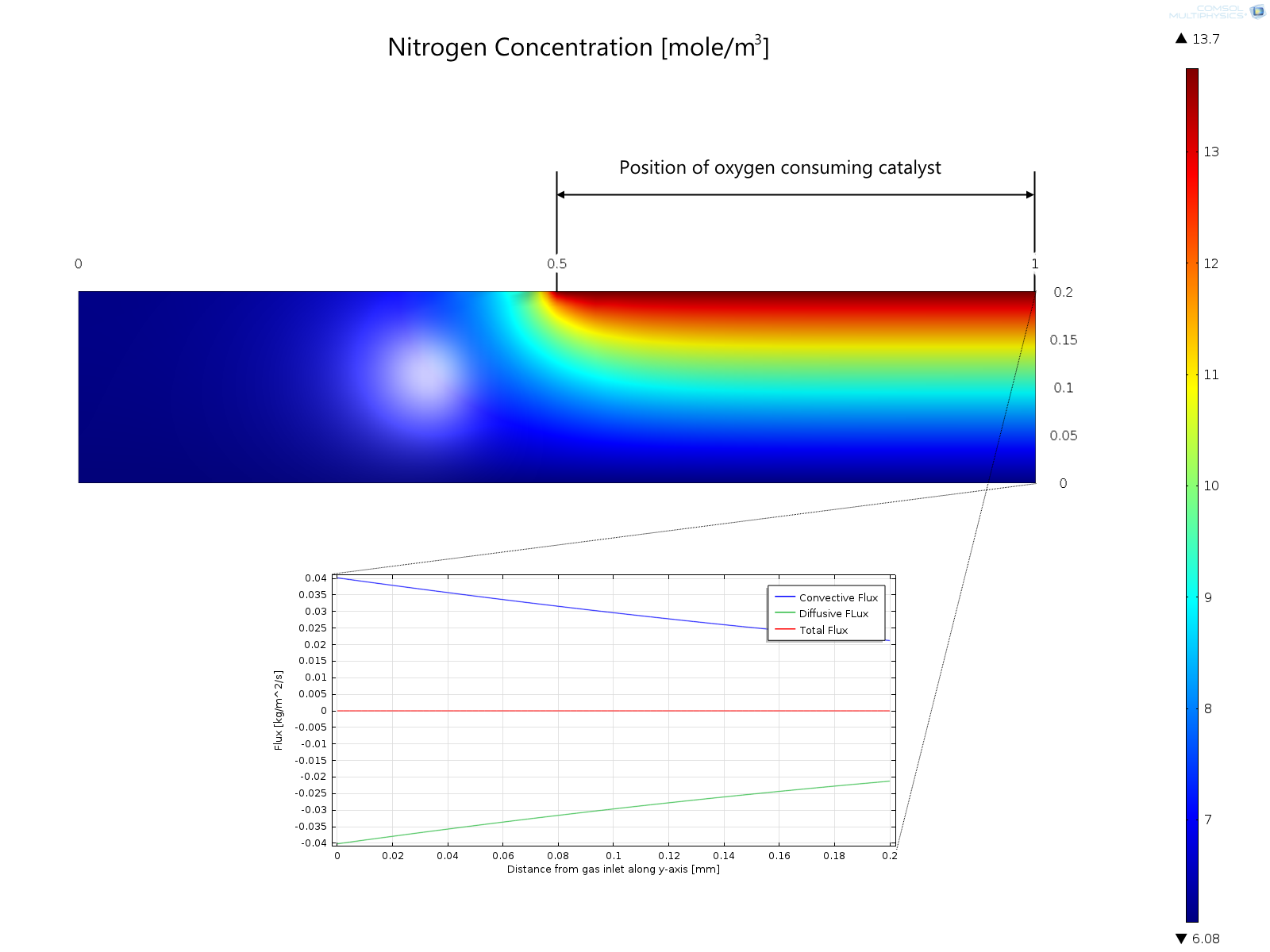 Surface plot of the nitrogen concentration in a gas diffusion electrode. The flux along the right vertical edge, plotted in the x-y plot, shows that the diffusive flux from the catalytic surface exactly compensates the convective flux to this surface, generated by oxygen consumption at the catalyst's surface.
Surface plot of the nitrogen concentration in a gas diffusion electrode. The flux along the right vertical edge, plotted in the x-y plot, shows that the diffusive flux from the catalytic surface exactly compensates the convective flux to this surface, generated by oxygen consumption at the catalyst's surface.
Surface plot of the nitrogen concentration in a gas diffusion electrode. The flux along the right vertical edge, plotted in the x-y plot, shows that the diffusive flux from the catalytic surface exactly compensates the convective flux to this surface, generated by oxygen consumption at the catalyst's surface.
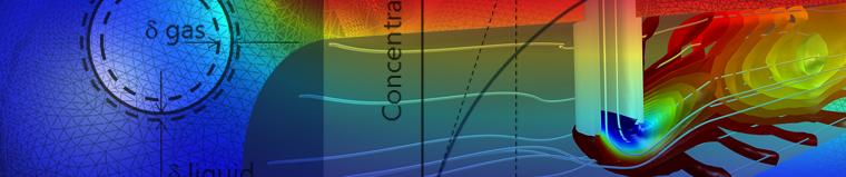
Due to the difficulties of numerically resolving steep gradients in potential, mass transfer across phase boundaries is often expressed using difference equations, instead of differential equations. This approximation implies that the gradients, included in the driving forces, are linearized inside a fictitious boundary layer (see the figure below). The thickness of the layer is then defined as the distance from a phase boundary where the linearized concentration gradient, starting from the concentration at the phase boundary, reaches the bulk concentration. The definition of the boundary layer also means that its thickness may be different for different species.
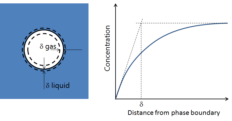 Fictive boundary layers inside and around a gas bubble in a liquid.
Fictive boundary layers inside and around a gas bubble in a liquid.
Fictive boundary layers inside and around a gas bubble in a liquid.
The mass transfer coefficient, km, for such an interface is defined as the diffusivity divided by the boundary layer thickness, δ.
(14)

An estimate of the relation between the boundary layer thickness and a system’s typical length is given by the Sherwood number:
(15)

In this expression, L denotes a typical length for a system, such as the radius of a pipe and the width of a channel. However, if the mass transport around a gas bubble in a liquid is studied, then L may denote the radius of the bubble. Since the thickness of the boundary layer depends on the convection just outside an interface, the Sherwood number also gives a measurement of the convective and diffusive fluxes to such an interface.
The boundary layer thickness at a liquid-gas interface for a rising bubble is of the order of magnitude of 100 μm in the gas phase and around 10 μm in the liquid phase.
The Sherwood number can also be defined as a function of the Reynolds and Schmidt numbers. The Reynolds number gives an estimate of the ratio of momentum transport by inertia to viscosity in a fluid:
(16)

where μ denotes viscosity and U denotes an average velocity. The Schmidt number gives an estimate of the relation between viscosity and diffusivity in a fluid:
(17)

The mass transfer coefficient can be estimated from the relation between the Sherwood number and the Reynolds and Schmidt numbers. For example, for forced convection along a flat plate, the following expression can be used:
(18)

where floc denotes the local friction factor for flow along a flat plate. The friction coefficient for different geometries is tabulated in literature and may also be obtained experimentally. All the material properties and the average velocity in the relation above are relatively easy to find in literature or estimate from simple calculations. Once the Sherwood number is calculated, then the mass transfer coefficient can be calculated, including the boundary layer thickness, which is the parameter that is not easily estimated otherwise. Note, though, that the above expression is only valid for flat plates.
Summary of Mass Transfer
The driving forces for mass transfer are relatively easy to define. These forces give the expressions for the flux, which can be used in the equations for conservation of mass. When these equations are discretized using a numerical method and when the resulting numerical model equations are solved, the results give the concentration distribution and fluxes in a system as functions of the modeled space coordinates and time. The estimates of the concentration and fluxes can be used to understand, design, optimize, and control the system that is being studied.
In cases where the equations cannot easily be discretized and solved in a detailed way, mass transfer coefficients may be used for obtaining an estimate of concentrations and fluxes in a system, which are less detailed than the one described above.
Published: January 14, 2015Last modified: February 22, 2017