
Introduction to Field Electromagnetics
What Is Electromagnetics?
As an engineering field, electromagnetics is traditionally approached through the jargon and devices belonging to one of many subfields, such as electrostatics or optics. A device used in an electrostatics setting, such as a capacitor, may have very little in common with one from optics, such as an optical fiber. Despite their widely differing characteristics, all of these application areas are fundamentally described by Maxwell's equations. In engineering applications, these equations almost always need to be supplemented by additional laws related to how electromagnetic fields interact with media. Maxwell's equations are listed in the table below in their differential form:
| Equation Name | Differential Form |
|---|---|
| Maxwell–Ampère's law |  |
| Faraday's law |  |
| Gauss's law |  |
| Gauss's magnetic law |  |
The meaning of these equations is described in the sections and subsections below.
In real-world applications, it is rarely necessary to consider all possible electromagnetic phenomena that may occur. Instead, a more practical understanding of electromagnetics comes from considering a number of special cases, including electrostatics, steady currents, magnetostatics, quasistatic alternating currents, inductive phenomena, microwave engineering, and optics.
Electrostatics
Electrostatics is the subfield of electromagnetics describing an electric field due to static (nonmoving) charges. As an approximation of Maxwell's equations, electrostatics can only be used to describe insulating, or dielectric, materials entirely characterized by the electric permittivity, sometimes referred to as the dielectric constant. When performing an electrostatics analysis, any conducting materials, typically metals, are first removed from the analysis, and the metallic surfaces are seen as exterior boundaries from the perspective of the dielectric materials. Typical inputs and outputs for an electrostatics analysis are summarized below:
| Inputs | Symbol | Geometric Location |
|---|---|---|
| Relative permittivity |  |
Volume |
| Electric potential |  |
Conducting boundary |
| Surface charge density |  |
Boundary |
| Volume charge density |  |
Volume |
| Polarization |  |
Volume |
| Outputs | Symbol | Geometric Location |
| Electric potential | |
Volume |
| Floating electric potential | |
Conducting boundary |
| Surface charge density | |
Conducting boundary |
| Electric field |  |
Volume |
| Electric displacement field |  |
Volume |
| Capacitance matrix |  |
Global |
| Electrostatic force |  |
Global |
Note that for an electrostatics analysis, there is no current input or output due to the fact that all charges are considered stationary. In certain cases, the volume charge density can also be an output of the analysis.
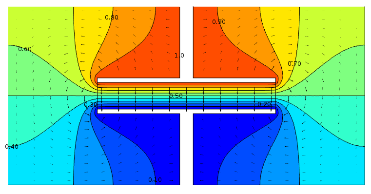
A cross-sectional view of the electric potential and field throughout the volume surrounding a parallel plate capacitor. The electric potential is visualized as filled contours with labels indicating the potential level. The electric field is visualized as logarithmically scaled arrows. The electric potential is also affected by the surrounding media further away and not shown in the picture.
A cross-sectional view of the electric potential and field throughout the volume surrounding a parallel plate capacitor. The electric potential is visualized as filled contours with labels indicating the potential level. The electric field is visualized as logarithmically scaled arrows. The electric potential is also affected by the surrounding media further away and not shown in the picture.
Typical applications of electrostatics analyses are capacitance calculations for capacitive devices and sensors such as touch screens, as well as dielectric strength evaluation of insulators, MEMS accelerometers, and MEMS gyroscopes.
Steady Currents
Steady currents analysis is used to compute the steady current flow in highly conductive materials such as metals. An electronic current is driven through a conductor by a difference in the electric potential. By convention and for historical reasons, the current flows from high potential to low potential values, although the electrons actually travel in the opposite direction of the current flow. The convention stems from the time before the discovery of the electron.
The material in a steady currents analysis is completely characterized by its electrical conductivity. When performing a steady currents analysis, any insulating materials are first removed from the analysis and the insulating surfaces are seen as exterior boundaries from the perspective of the conductive materials.
Typical inputs and outputs for a steady currents analysis are summarized below:
| Input | Symbol | Geometric Location |
|---|---|---|
| Conductivity or resistivity |  , , |
Volume |
| Electric potential | |
Boundary |
| Normal current density |  |
Boundary |
| Output | Symbol | Geometric Location |
| Electric potential | |
Volume |
| Floating electric potential | |
Conducting boundary |
| Normal current density | |
Boundary |
| Electric field | |
Volume |
| Current density |  |
Volume |
| Resistance matrix |  |
Global |
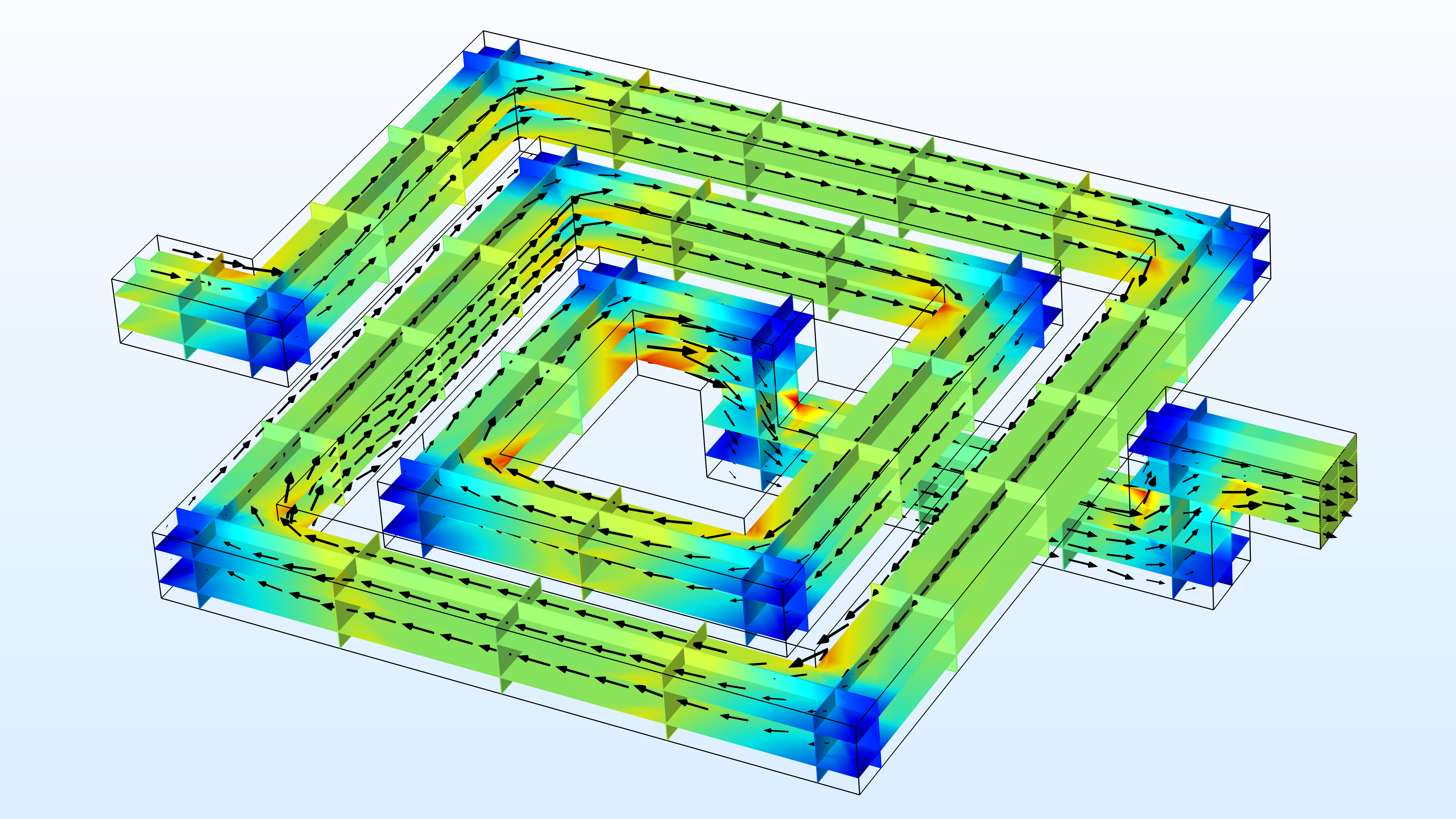
The current density in a spiral inductor where a potential difference is applied between the left and right boundaries. The picture shows the current density magnitude values inside the inductor. Blue and red represent low and high magnitude values, respectively. The arrows show the direction of the current density. The tendency of the current to take the shortest path is visible as red areas in the inner corners of the structure.
The current density in a spiral inductor where a potential difference is applied between the left and right boundaries. The picture shows the current density magnitude values inside the inductor. Blue and red represent low and high magnitude values, respectively. The arrows show the direction of the current density. The tendency of the current to take the shortest path is visible as red areas in the inner corners of the structure.
Typical applications of steady currents analysis are electronic components, electrical cables, high-voltage system components, medical devices, sensors, geotechnical analysis, and corrosion.
Electroquasistatics
Electroquasistatics analysis is a generalization of electrostatics and steady currents in cases where magnetic effects can be neglected. It is only possible to combine the capacitive effects of electrostatics with the conductive effects of a steady currents analysis if the fields are time varying. One can say that for the static case, Maxwell's equations split into the electrostatics and steady currents cases, and one has to choose one of them, as they represent mutually exclusive phenomena. However, if there is any time variation in, say, voltages at the boundaries, the total current is the sum of a conduction current and a displacement current. The conduction current density is associated with the electric conductivity, and the displacement current density is associated with the electric permittivity. Electroquasistatics can be seen as a dynamic version of the steady currents equations with an additional contribution from the displacement current. For a time-harmonic analysis, where the driving current or voltage is sinusoidal, the fields become complex-valued where the phase angle represents the ratio between conduction and displacement currents.
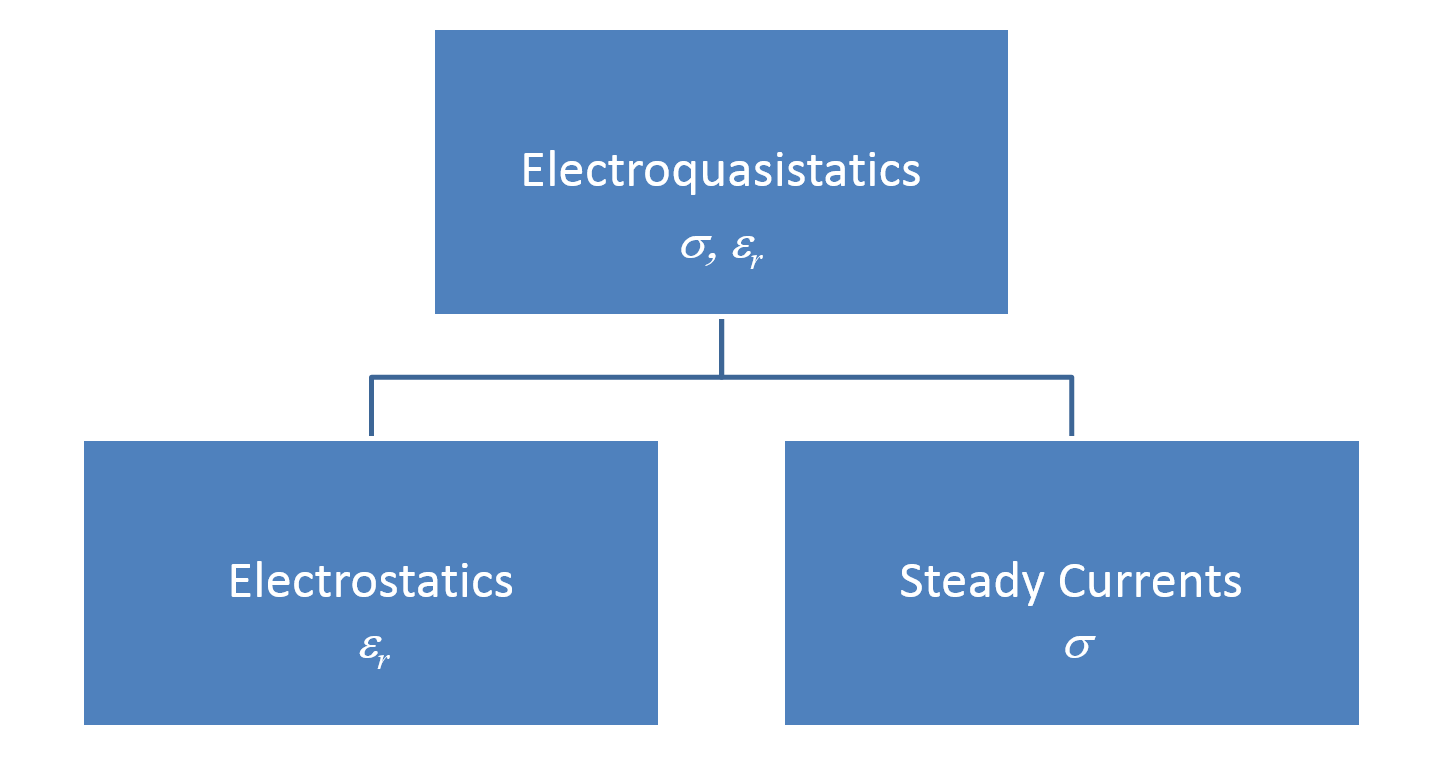
Electroquasistatics is a generalization of electrostatics and steady currents for time-varying fields where magnetic effects can be neglected.
Electroquasistatics is a generalization of electrostatics and steady currents for time-varying fields where magnetic effects can be neglected.
Typical inputs and outputs for an electroquasistatics analysis are summarized below:
| Inputs | Symbol | Geometric Location |
|---|---|---|
| Conductivity or resistivity | , |
Volume |
| Relative permittivity | |
Volume |
| Electric potential | |
Boundary |
| Normal current density | |
Boundary |
| Outputs | Symbol | Geometric Location |
| Electric potential | |
Volume |
| Floating electric potential | |
Conducting boundary |
| Normal current density | |
Boundary |
| Electric field | |
Volume |
| Current density | |
Volume |
| Resistance matrix |  |
Global |
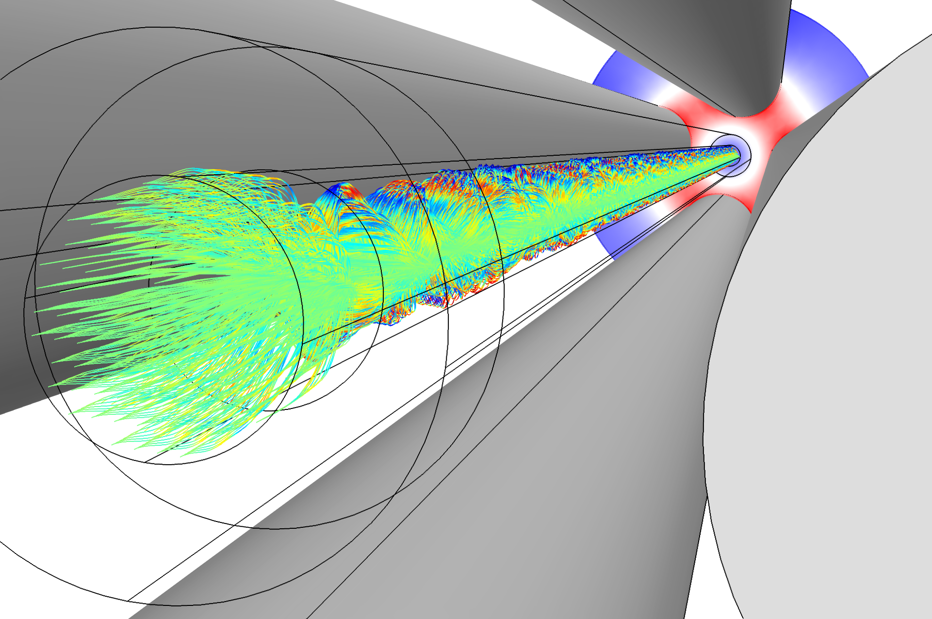
The ion trajectories in a quadrupole mass spectrometer. This type of spectrometer sorts particles by using a clever combination of static and time-harmonic electric potential. By tuning the harmonic frequency (here at 4 MHz) and the strengths of the static and harmonic fields, only particles of a certain mass are transmitted through the device.
The ion trajectories in a quadrupole mass spectrometer. This type of spectrometer sorts particles by using a clever combination of static and time-harmonic electric potential. By tuning the harmonic frequency (here at 4 MHz) and the strengths of the static and harmonic fields, only particles of a certain mass are transmitted through the device.
Typical applications where electroquasistatics analysis is useful include medical devices, sensors, geotechnical analysis, and mass spectrometers.
To learn more about the theory of electroquasistatics, see Electroquasistatics, Theory.
Magnetostatics
Magnetostatics can be seen as a magnetic generalization of steady currents and is used when information of the magnetic field that surrounds a conductor is needed. In this context, a steady currents analysis is sometimes used as a preprocessing step, and the resulting currents are used as input to a subsequent magnetostatics analysis. This would be the case, for example, when analyzing an electromagnet. The fundamental material property for performing a magnetostatics analysis is the relative permeability. For nonlinear magnetostatics analyses, a more general material relationship may be needed, such as a functional relationship between the magnetic field and the magnetic flux density: a so-called B-H curve. The ultimate goal of a magnetostatics analysis is, in many cases, to compute the mutual inductance and self inductance of a system of coils or the forces and torques in a system of magnetic components.
Analysis of permanent magnets constitutes an important, special case of magnetostatics analysis. In this case, a permanent magnetization is the source of the magnetic field instead of an electrical current. In such cases, the magnetic flux strength and direction as well as forces are important analysis results.
Magnetostatics can be seen as a generalization of steady currents and is used when information about magnetic fields is needed.
Magnetostatics can be seen as a generalization of steady currents and is used when information about magnetic fields is needed.
Typical inputs and outputs for a magnetostatics analysis are summarized below:
| Inputs | Symbol | Geometric Location |
|---|---|---|
| Conductivity or resistivity | , |
Volume |
| Relative permeability |  |
Volume |
| B-H curve |  |
Volume |
| Current density in coils | |
Volume |
| Magnetic field |  |
Boundary |
| Current density on surface and edges |  |
Boundary |
| Outputs | Symbol | Geometric Location |
| Magnetic field | |
Volume |
| Magnetic flux |  |
Volume |
| Inductance matrix |  |
Global |
| Magnetic force | |
Global |

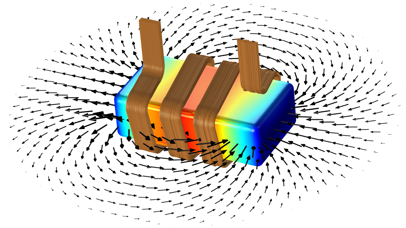
Magnetic flux lines surrounding an inductor carrying a steady current.
Magnetic flux lines surrounding an inductor carrying a steady current.
Visualization of the magnetic flux in a system consisting of a horseshoe magnet and an iron rod.
Visualization of the magnetic flux in a system consisting of a horseshoe magnet and an iron rod.
Typical applications where magnetostatics analysis is useful include electromagnets, permanent magnets, coils, inductors, and solenoids.
To learn more about the theory of magnetostatics, see Magnetostatics, Theory.
Magnetoquasistatics
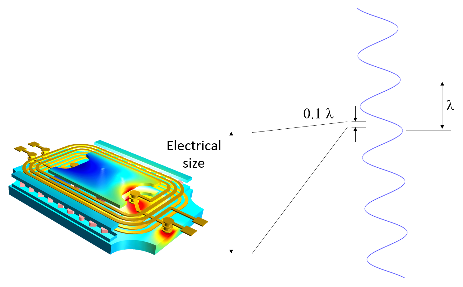
A consequence of Maxwell’s equations is that changes in time, of currents and charges, are not synchronized with changes of the electromagnetic fields. The changes of the fields are always delayed relative to the changes of the sources, reflecting the finite speed of propagation of electromagnetic waves. Under the assumption that this effect can be ignored, it is possible to obtain the electromagnetic fields by considering "stationary currents at every instant". This low-frequency approximation is valid, provided that the variations in time are small enough and that the studied geometries are considerably smaller than the wavelength. As a rule of thumb, the quasistatic approximation can be used when the characteristic size of a device, the electrical size, is smaller than 10% of the wavelength.
The magnetoquasistatics approximation is very important for understanding electromagnetic components in 50-Hz or 60-Hz power grid networks. This class of analysis is also important for higher frequencies and is sometimes combined with a full electromagnetic wave analysis for assessing electromagnetic interference phenomena.
For linear material properties and sinusoidal currents and fields, time-harmonic studies are used. Such studies are very efficient, as the components can be analyzed for one frequency at a time and the full behavior for all times is captured in one go. For components with nonlinear materials or distorted wave forms, a full time-dependent analysis is needed, which can lead to long computation times.
The excitation of magnetoquasistatic components is done with time-varying voltages or currents at the boundaries of the domain of interest or as volumetric coil currents. Such methods of excitation are only valid in the low-frequency regime. At higher frequencies, radiation losses and effects stemming from the finite speed of light become important, and a high-frequency analysis may become necessary.
Typical inputs and outputs for a magnetoquasistatic analysis are summarized below:
| Inputs | Symbol | Geometric Location |
|---|---|---|
| Conductivity or resistivity | , |
Volume |
| Relative permittivity | |
Volume |
| Relative permeability | |
Volume |
| B-H curve | |
Volume |
| Current density in coils | |
Volume |
| Magnetic field | |
Boundary |
| Current density on surfaces and edges |
|
Boundary |
| Outputs | Symbol | Geometric Location |
| Magnetic field | |
Volume |
| Magnetic flux | |
Volume |
| Impedance matrix | |
Global |
A 50-Hz AC coil wound around a ferromagnetic core.
A 50-Hz AC coil wound around a ferromagnetic core.
Typical magnetoquasistatics applications include cables, power lines, transformers, generators, motors, reactive ballasts, inductors, and capacitors.
Electromagnetic Waves
James Clark Maxwell generalized Ampère's law by adding a term for the displacement current, discovering the equation now known as Maxwell–Ampère's law. By combining it with Faraday's law, he discovered the wave nature of electromagnetic phenomena represented by the electromagnetic wave equation. There are several formulations of the electromagnetic wave equation, such as the one in terms of the electric field:

and similarly for the magnetic field:

This led Maxwell to conclude, among other things, that the speed of light is universal for all electromagnetic phenomena. The speed of light is related to the permittivity and permeability according to:

The continuum approach to analyzing electromagnetic phenomena has proven very successful for many applications, but it comes with certain limitations. For microscopic structures where the discrete nature of matter becomes important, a quantum mechanical approach is required. For very high frequencies, the electromagnetic waves can more efficiently be analyzed as rays, and for even higher frequencies, the individual photons have to be modeled together with their ionizing interaction with matter.
To determine the appropriate method of electromagnetics analysis, one has to consider the relative relationship between the object's characteristic size and the wavelength. The following diagram gives an overview of this relationship.
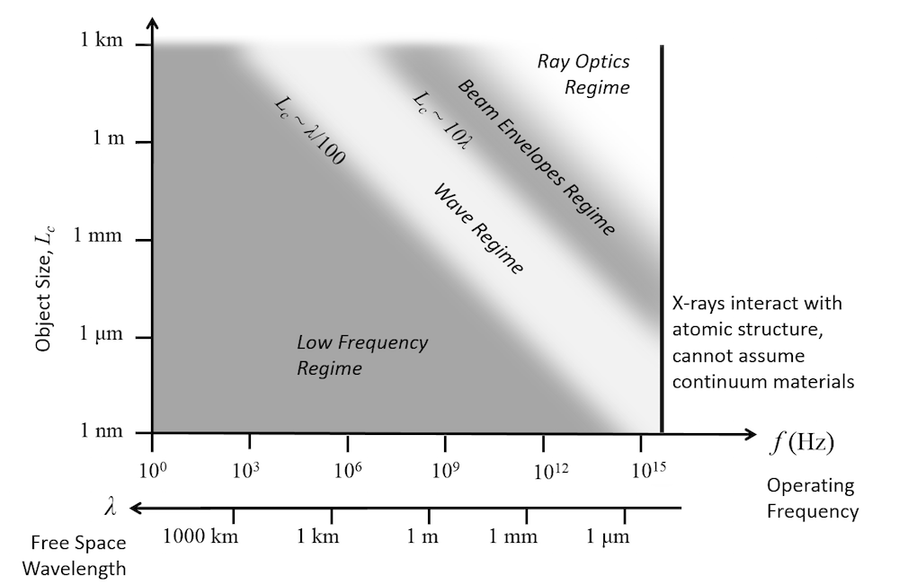
The size of an object relative to the wavelength is illustrated together with the preferred analysis method.
The size of an object relative to the wavelength is illustrated together with the preferred analysis method.
The wave nature of electromagnetic fields is important to analyze for devices that are either guiding or radiating electromagnetic waves. This includes, for example, coaxial cables, microwave circuits, waveguides, and antennas.
At high frequencies, the effects of the finite speed of light become important, and quantities like voltages are no longer constant over boundary segments and cannot be used directly for the excitation of devices. Instead, field patterns, eigenmodes that are compatible with Maxwell's equations, are used on so-called ports or port boundaries. Used correctly, these types of boundary conditions can excite structures with very small losses and thus capture their intrinsic performance under ideal conditions.
It can sometimes be convenient to use an engineering approach with voltage and current excitations representing the feed from adjoined electrical circuits. These can be used together with elaborate schemes for conversions into compatible port excitations. In such cases, energy losses are inevitable and may represent real device feed losses, artificial modeling losses, or both. In a similar way, so-called listening ports are used to transmit outgoing energy in a way that is consistent with Maxwell's equations. The transmitted and reflected energy is computed as so-called scattering parameters, or S-parameters, which represent the input and output of energy through the various ports.
Typical inputs and outputs for an electromagnetic wave analysis are summarized below:
| Inputs | Symbol | Geometric Location |
|---|---|---|
| Conductivity or resistivity | , |
Volume |
| Relative permittivity | |
Volume |
| Relative permeability | |
Volume |
Input power for port  |
 |
Boundary |
| Phase for port |
 |
Boundary |
| Feed circuit voltage or current |
 |
Boundary |
| Outputs | Symbol | Geometric Location |
| Electric field | |
Volume |
| Magnetic field | |
Volume |
| Impedance matrix | |
Global |
| Admittance matrix |  |
Global |
| S-parameter matrix |  |
Global |
| Antenna parameters | No convention | Global |
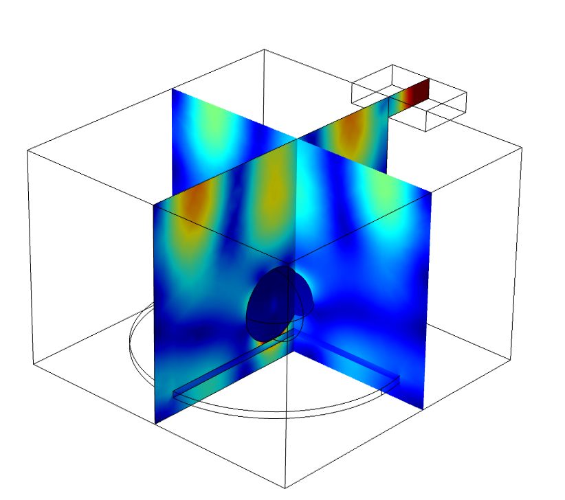
The standing electromagnetic wave in a household microwave oven.
The standing electromagnetic wave in a household microwave oven.
To learn more about the theory of electromagnetic waves, see Electromagnetic Waves, Theory.
Electromagnetic Heating
Joule Heating
Joule heating (also referred to as resistive or ohmic heating) describes the process in which the energy of an electric current is converted into heat as it flows through a resistance.
In particular, when the electric current flows through a solid or liquid with finite conductivity, electric energy is converted to heat through resistive losses in the material. The heat is generated on the microscale when the conduction electrons transfer energy to the conductor's atoms by way of collisions.
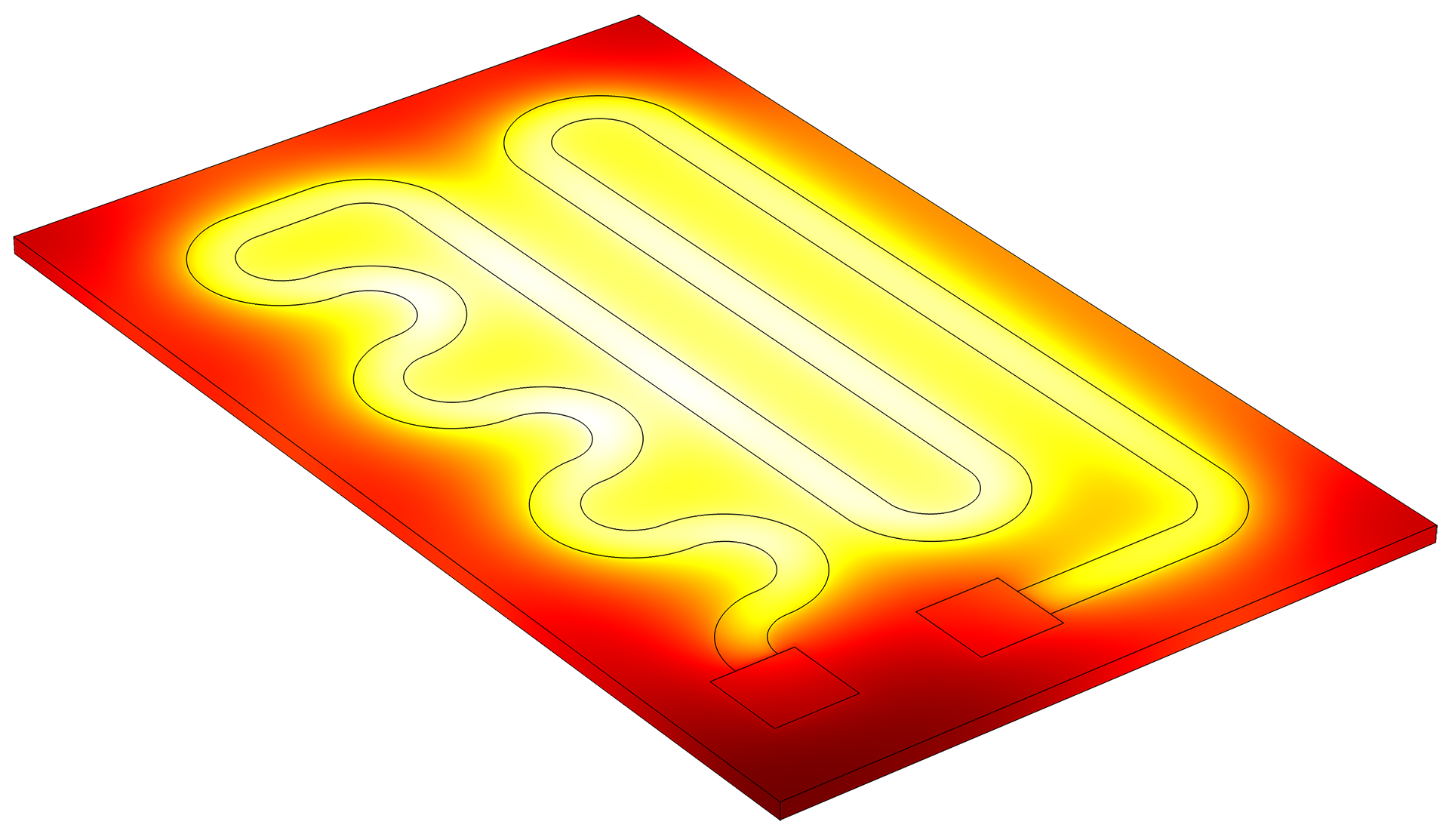
A heating circuit, showing temperature distribution as a result of Joule heating.
A heating circuit, showing temperature distribution as a result of Joule heating.
In some cases, Joule heating is pertinent to an electrical device's design, while in others, it is an unwanted effect. A couple of applications that do rely on Joule heating include hot plates (directly) and microvalves for fluid control (indirectly, through thermal expansion).
In the event that the effect is undesirable in a design, efforts can be made to reduce it. Joule heating is particularly relevant in terms of electrical system components, such as conductors in electronics, electric heaters, power lines, and fuses. The heating of these structures can cause them to degenerate or even melt. To prevent the components and devices from overheating, engineers can incorporate convection cooling into the design.
Below is an example of mechanical stress induced in a heating circuit by way of Joule heating. Upon applying a voltage to the circuit, the electrically conductive layer over the glass plate causes Joule heating. This, in turn, impacts the structural integrity of the circuit and induces bending of the glass plate.
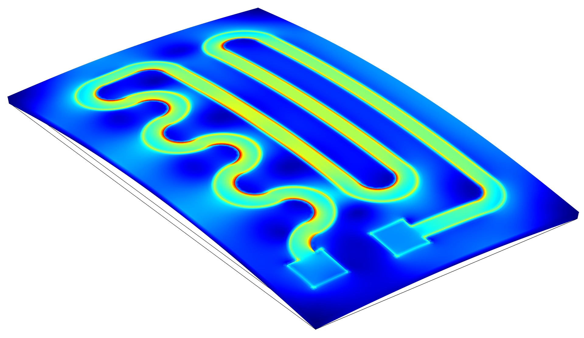
A heating circuit. The stress is highest in the red areas. The glass plate in the circuit bends due to the heat imposed on the plate and the expansion of the circuit.
A heating circuit. The stress is highest in the red areas. The glass plate in the circuit bends due to the heat imposed on the plate and the expansion of the circuit.
Typical inputs and outputs for a Joule heating analysis are summarized below:
| Inputs | Symbol | Geometric Location |
|---|---|---|
| Conductivity or resistivity | , |
Volume |
| Electric potential | |
Boundary |
| Normal current density | |
Boundary |
| Thermal conductivity |  |
Volume |
| Heat capacity |  |
Volume |
| Mass density | |
Volume |
| Temperature |  |
Boundary |
| Heat flux |  |
Boundary |
| Outputs | Symbol | Geometric Location |
| Electric potential | |
Volume |
| Current density | |
Volume |
| Power dissipation |  |
Volume |
| Temperature | |
Volume |
| Heat flux | |
Volume |
Induction Heating
Induction heating is similar to the Joule heating effect, but with one important modification: The currents that heat the material are induced by means of electromagnetic induction; it is a no-contact, or nonlocal, heating process.
By applying a high-frequency alternating current to an induction coil, a time-varying magnetic field is generated. The material to be heated, known as the workpiece, is placed inside the magnetic field without touching the coil. Note that not all materials can be heated by induction; only those with high electrical conductivity (such as copper, gold, and aluminum, to name a few). The alternating electromagnetic field induces eddy currents in the workpiece, resulting in resistive losses, which then heat up the material.

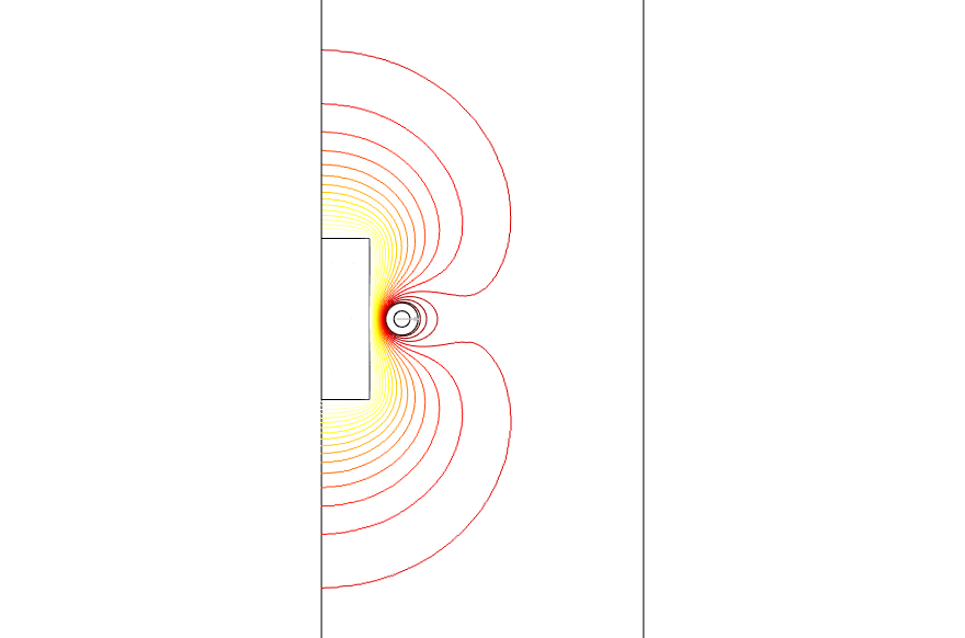
Induced current density in a copper plate at 10 Hz.
Induced current density in a copper plate at 10 Hz.
Furthermore, the high frequency leads to a skin effect. The alternating current is forced to flow in a thin layer toward the surface of the workpiece. This in turn leads to an increased resistance of the conductor, ultimately resulting in a greatly increased heating effect.
Ferrous metals are heated by induction more easily than other materials. This is because their high permeability boosts the induced eddy currents and skin effect. In addition, another heating mechanism occurs. The material's iron crystals are magnetized and demagnetized over and over by the alternating magnetic field. This causes the magnetic domains to flip rapidly back and forth, leading to hysteresis losses, which result in additional heat.
So, induction heating takes place without physical contact between the workpiece and induction coil. This lends it to processes where a high degree of cleanliness is paramount, such as in semiconductor manufacturing.

Magnetic flux density.
Magnetic flux density.
Additionally, this method of heating is very efficient, as the heat is generated inside the workpiece, as opposed to somewhere else and then applied to the workpiece. In other words, with induction heating, we can avoid heat losses from the surfaces that would provide the electrical connection, thus improving the overall heating efficiency.
Induction heating involves two different types of physics: electromagnetism and heat transfer. Some material properties are temperature dependent, meaning they change when heat is applied. In that event, you can consider the two physical phenomena coupled.
Skin effect: The current density is high near the surface of the conductor.
Skin effect: The current density is high near the surface of the conductor.
One innovation that takes advantage of induction heating is the induction stove. In this design, the coil is placed beneath the stovetop and its electromagnetic fields act on the metal pot. Since only highly conductive materials can be heated this way, the pot heats up, while if you placed your hand on the stove top, it would not feel hot.
The semiconductor industry also makes use of this process for heating silicon. Other applications include sealing, heat treatment, and welding.
Temperature plot of induction heating in a copper cylinder.
Temperature plot of induction heating in a copper cylinder.
While there are plenty of products and processes that function thanks to induction heating, there is one application where heating leads to wasted power. When it comes to transformers, it is important not to allow eddy currents to flow inside the cores. If eddy currents heat the transformer's magnetic core, power is wasted and further problems could occur, such as structural damage.
Typical inputs and outputs for an induction heating analysis are summarized below:
| Inputs | Symbol | Geometric Location |
|---|---|---|
| Conductivity or resistivity | ,  |
Volume |
| Relative permeability | |
Volume |
| Coil current |  |
Volume |
| Thermal conductivity | |
Volume |
| Heat capacity | |
Volume |
| Mass density | |
Volume |
| Temperature | |
Boundary |
| Heat flux | |
Boundary |
| Outputs | Symbol | Geometric Location |
| Electric field | |
Volume |
| Magnetic flux | |
Volume |
| Induced current density |  |
Volume |
| Power dissipation | |
Volume |
| Temperature | |
Volume |
| Heat flux | |
Volume |
Microwave Heating
Microwave heating is a multiphysics phenomenon that involves electromagnetic waves and heat transfer. Any material that is exposed to electromagnetic radiation will be heated up. The rapidly varying electric and magnetic fields lead to four sources of heating. Any electric field applied to a conductive material will cause current to flow. In addition, a time-varying electric field will cause dipolar molecules, such as water, to oscillate back and forth. A time-varying magnetic field applied to a conductive material will also induce current flow. There can also be hysteresis losses in certain types of magnetic materials.
One obvious example of microwave heating is in a microwave oven. When you place food in a microwave oven and press the "start" button, electromagnetic waves oscillate within the oven at a frequency of 2.45 GHz. These fields interact with the food, leading to heat generation and a rise in temperature.
The electric field and temperature plot for a tutorial model of a microwave oven cooking a potato. The rectangular block on the right represents a waveguide feed.
The electric field and temperature plot for a tutorial model of a microwave oven cooking a potato. The rectangular block on the right represents a waveguide feed.
The efficiency of microwave heating depends on the material properties. For example, if you place foods with varying water content in a microwave oven, they will heat up at different rates. A dinner plate may come out with some food on it that is very hot, while the rest of it is still cold. Furthermore, the position of food items relative to each other will also affect the electromagnetic field within the oven. That is why most microwave ovens have turntables to rotate the food and promote even heating.
Another application that leverages the effects of microwave heating is cancer treatment, in particular, hyperthermic oncology. This type of cancer therapy involves subjecting tumor tissue to localized heating without damaging the healthy tissue around it. Doctors performing microwave coagulation therapy insert a thin microwave antenna directly into the tumor and heat it up. The microwave heating generates a coagulated region, killing the cancerous cells. This treatment method requires controlling the spatial distribution and heating power. The temperature sensors must be both well designed and strategically placed in order to avoid harming healthy tissue.
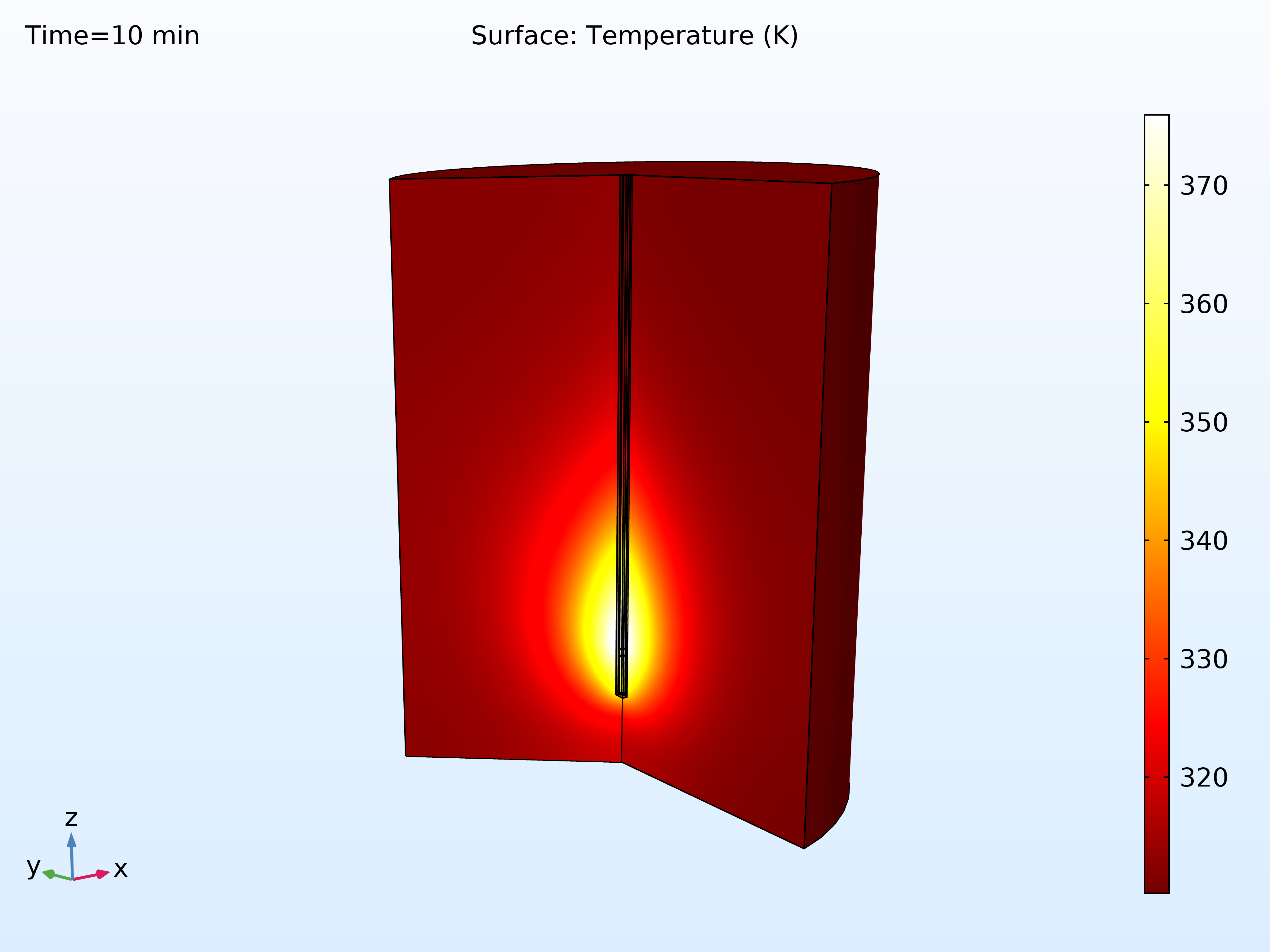
Microwave heating of liver tissue for cancer treatment.
Microwave heating of liver tissue for cancer treatment.
Typical inputs and outputs for a microwave heating analysis are summarized below:
| Inputs | Symbol | Geometric Location |
|---|---|---|
| Conductivity or resistivity | , |
Volume |
| Relative permeability | |
Volume |
| Relative permittivity | |
Volume |
| Import power for port |
|
Boundary |
| Feed circuit voltage or current | |
Boundary |
| Thermal conductivity | |
Volume |
| Heat capacity | |
Volume |
| Mass density | |
Volume |
| Temperature | |
Boundary |
| Heat flux | |
Boundary |
| Outputs | Symbol | Geometric Location |
| Electric field | |
Volume |
| Magnetic field | |
Volume |
| Induced current density | |
Volume |
| Power dissipation | |
Volume |
| Temperature | |
Volume |
| Heat flux | |
Volume |
Electromagnetic Forces
Electromagnetic forces can be categorized depending on their subfield of electromagnetics. Although the fundamental electromagnetic force is the same for all of them, their characteristic features and methods of computation are quite different. The most important types of electromagnetic forces are summarized in the table below:
| Force | Subfield | Typically Acts On | How to Compute Net Force |
|---|---|---|---|
| Electrostatic force | Electrostatics | Boundary | Integration on boundary |
| Dielectrophoretic force | Electrostatics and electroquasistatics | Particle | Analytical expression |
| Magnetostatic force | Magnetostatics | Boundary | Integration on boundary |
| Lorentz force | Magnetoquasistatics | Volume | Integration in volume |
| Radiation pressure | Electromagnetic waves | Boundary | Integration on boundary |
Electromagnetic forces are used in many industrial devices, including electromagnetic motors and generators, electromagnets, relays, electromagnetic valves, circuit breakers, plungers, and contactors.
Electromagnetic forces are not only of importance in solid materials. For example, in metals processing using induction furnaces, electromagnetic forces are important to understand, since molten metals are typically highly conductive. The area that combines magnetics and fluid flow is known as magnetohydrodynamics.

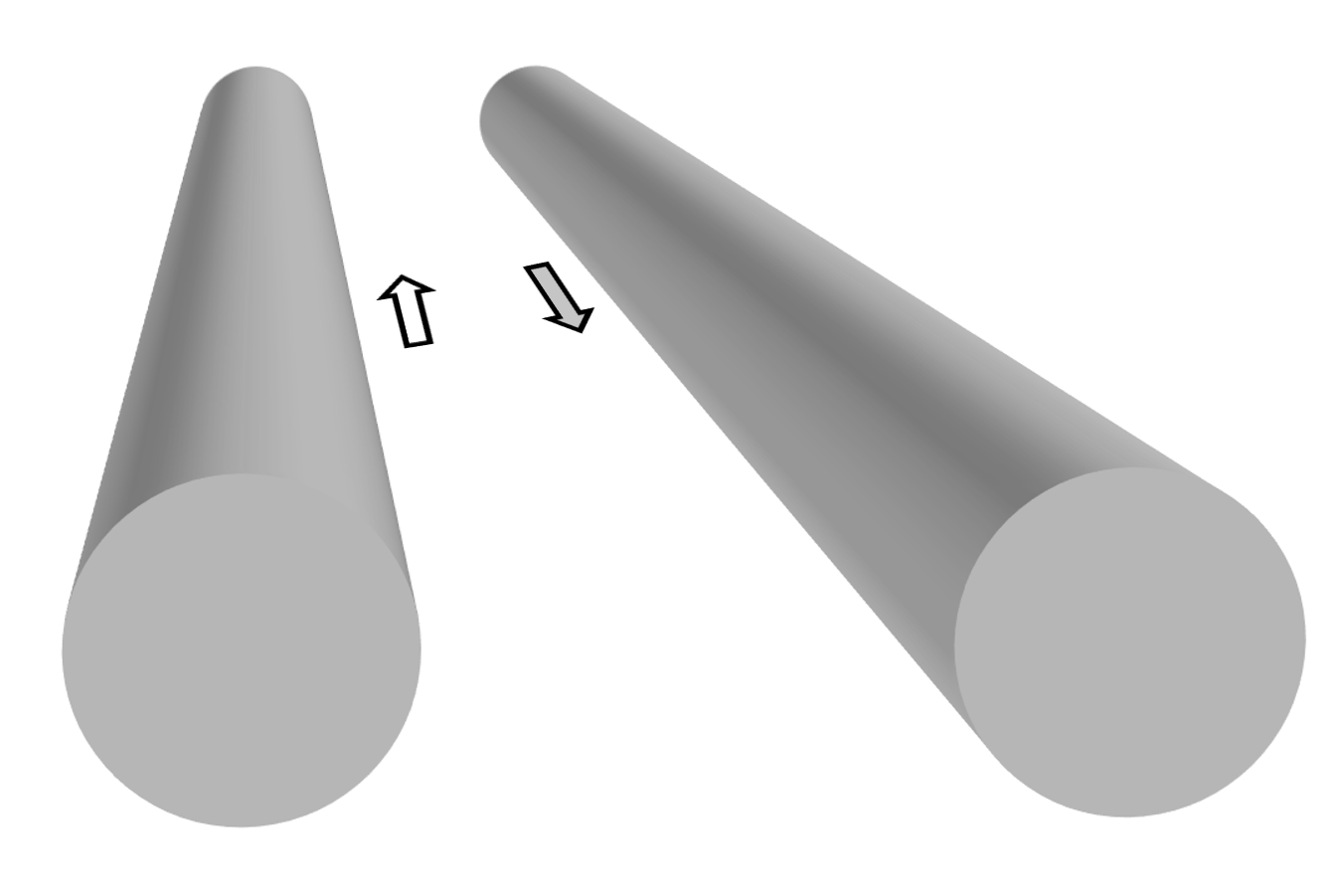
Linear electromagnetic actuators are useful in many industrial applications that require a linear motion, for example, to open or close and push or pull a load.
Linear electromagnetic actuators are useful in many industrial applications that require a linear motion, for example, to open or close and push or pull a load.
Magnetostatic Force
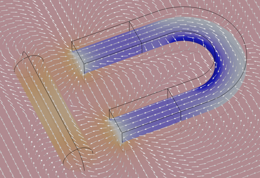
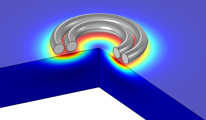
Magnetostatic forces are perhaps the most familiar electromagnetic forces in everyday life, with the omnipresence of permanent magnets. These are found in refrigerator magnets, latches for bags and wallets, magnetic connectors for power adapters and laptop keyboards, and so on. A classic example of a permanent magnet is the horseshoe magnet, as shown in the picture below. The magnetic forces in this case manifest as a surface force density stemming from the discontinuous jump in magnetic permeability when going from the interior of the permanent magnet out into the nonmagnetic surrounding air.
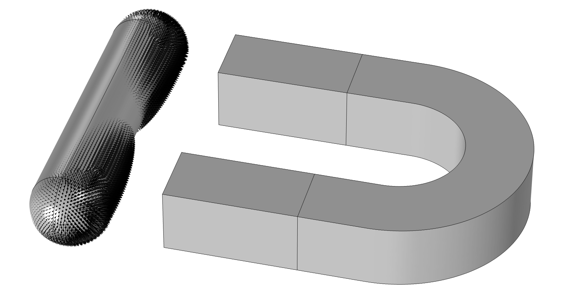
The magnetostatic force density at the surface of an iron rod adjacent to a horseshoe permanent magnet. The surface force density is visualized as black arrows.
The magnetostatic force density at the surface of an iron rod adjacent to a horseshoe permanent magnet. The surface force density is visualized as black arrows.
Electrostatic Force
In a similar way to magnetostatic forces, electrostatic forces often manifest as surface forces. Electrostatic forces are of importance in MEMS devices, either as wanted or unwanted forces.
Electrostatic forces are important when designing MEMS devices such as accelerometers.
Electrostatic forces are important when designing MEMS devices such as accelerometers.
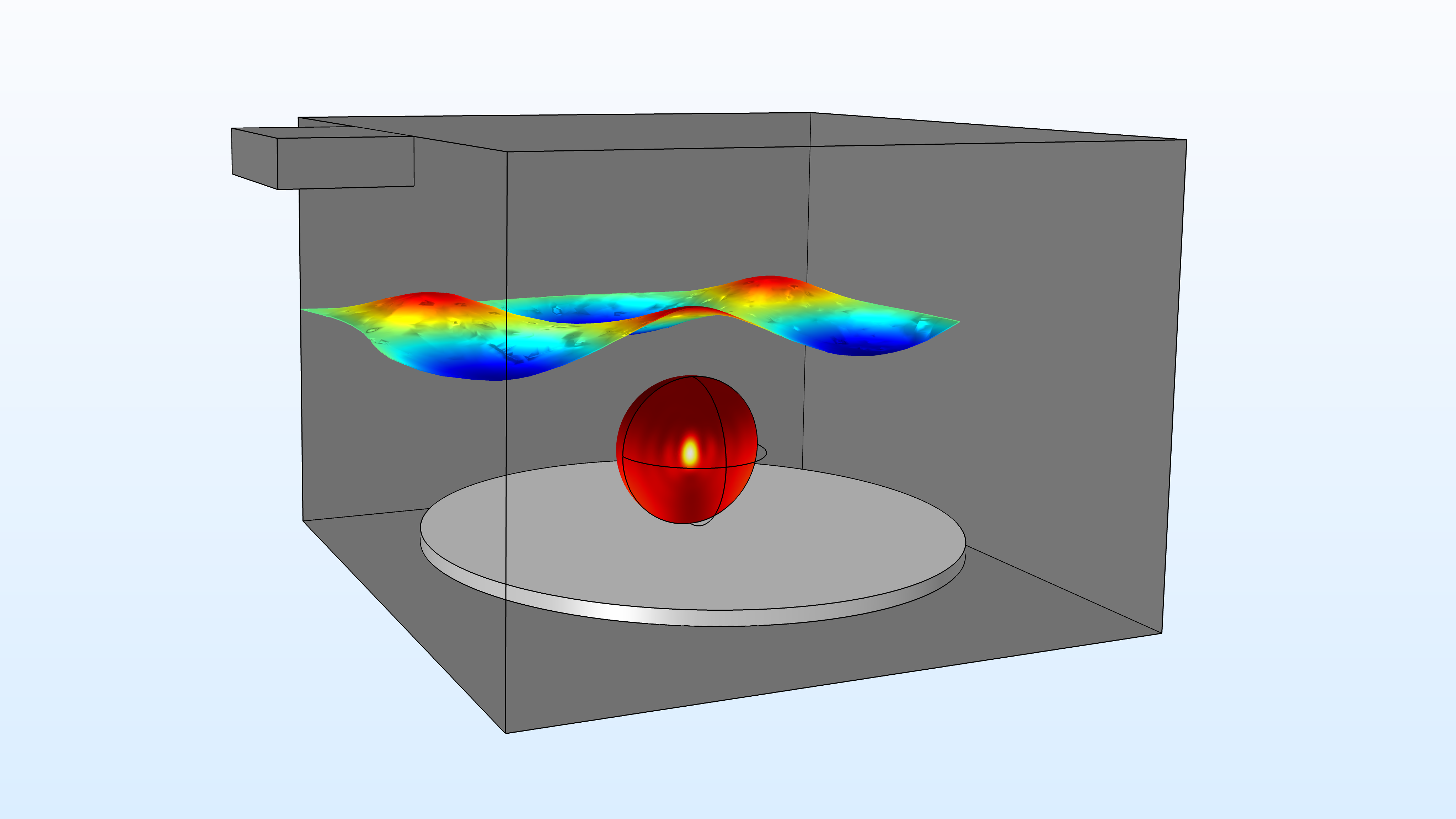
Lorentz Force
Lorentz forces are present whenever there is a current according to the well-known formula

where is the current density, is the magnetic flux, and  is the force density.
The magnetic flux can be generated directly or indirectly by the current , but can also be an externally generated magnetic flux.
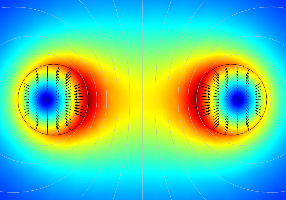
The Lorentz force density inside of two current-carrying wires with steady currents flowing in opposing directions. The force density is visualized on a cross section of the wires and the surrounding air by black arrows and the magnetic flux is visualized by color (magnitude) and contours. The Lorentz force density in one of the wires has contributions from both the self-induced magnetic field and the magnetic field from the adjacent wire. The net force here is repulsive.
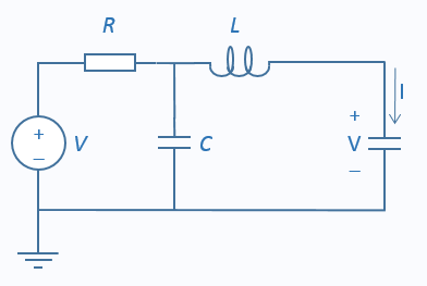
Lumped Circuit Parameters
In the area of electrical circuits, the fundamental quantities are not the electric or magnetic fields but rather lumped circuit parameters such as resistance and impedance. These circuit parameters typically describe the relationships between voltages and currents and encode system-level information about electromagnetic devices.
Last modified: April 3, 2019